Chapter 1 The Integrated Nested Laplace Approximation and the R-INLA package

1.1 Introduction

In this introductory chapter a brief summary of the integrated nested Laplace approximation (INLA, Rue, Martino, and Chopin 2009) is provided. The aim of this chapter is to introduce the INLA methodology and the main features of the associated INLA package (also called R-INLA) for the R programming language. Different models will be fitted to a simulated dataset in order to show the main steps to fit a model with the INLA methodology and the INLA package.

This introduction to INLA and the INLA package covers the basics as well as some advanced features. The aim is to provide the reader with a general overview that will be useful to follow the other chapters in the book on spatial models with the SPDE methodology. Other recent works that describe INLA are the following: Blangiardo and Cameletti (2015) provide an introduction to the main INLA theory and an extensive description of many spatial and spatio-temporal models. Wang, Faraway, and Yue Ryan (2018) provide a detailed description of INLA with a focus on general regression models. Similarly, Gómez-Rubio (2019) describes the underlying INLA methodology and describes many different models and computational aspects.

1.2 The INLA method

Rue, Martino, and Chopin (2009) develop the integrated nested Laplace approximation (INLA) for approximate Bayesian inference as an alternative to traditional Markov chain Monte Carlo (MCMC, Gilks, Richardson, and Spiegelhalter 1996) methods. INLA focuses on models that can be expressed as latent Gaussian Markov random fields (GMRF) because of their computational properties (see Rue and Held 2005 for details). Not surprisingly, this covers a wide range of models and recent reviews of INLA and its applications can be found in Rue et al. (2017) and Bakka et al. (2018).

The INLA framework can be described as follows. First of all, \(\mathbf{y}=(y_1,\ldots,y_n)\) is a vector of observed variables whose distribution is in the exponential family (in most cases), and the mean \(\mu_i\) (for observation \(y_i\)) is conveniently linked to the linear predictor \(\eta_i\) using an appropriate link function (it is also possible to link the predictor to e.g. a quantile). The linear predictor can include terms on covariates (i.e., fixed effects) and different types of random effects. The vector of all latent effects will be denoted by \(\mathbf{x}\), and it will include the linear predictor, coefficients of the covariates, etc. In addition, the distribution of \(\mathbf{y}\) will likely depend on some vector of hyperparameters \(\btheta_1\).

The distribution of the vector of latent effects \(\mathbf{x}\) is assumed to be Gaussian Markov random field (GMRF). This GMRF will have a zero mean and precision matrix \(\mathbf{Q}(\btheta_2)\), with \(\btheta_2\) a vector of hyperparameters. The vector of all hyperparameters in the model will be denoted by \(\btheta = (\btheta_1, \btheta_2)\).

Furthermore, observations are assumed to be independent given the vector of latent effects and the hyperparameters. This means that the likelihood can be written as

\[ \pi(\mathbf{y}|\mathbf{x},\btheta) =\prod_{i\in \mathcal{I}} \pi(y_i|\eta_i,\btheta). \]

Here, \(\eta_i\) is the latent linear predictor (which is part of the vector \(\mathbf{x}\) of latent effects) and set \(\mathcal{I}\) contains indices for all observed values of \(\mathbf{y}\). Some of the values may not have been observed.

The aim of the INLA methodology is to approximate the posterior marginals of the model effects and hyperparameters. This is achieved by exploiting the computational properties of GMRF and the Laplace approximation for multidimensional integration.

The joint posterior distribution of the effects and hyperparameters can be expressed as:

\[\begin{eqnarray} \pi(\mathbf{x}, \btheta|\mathbf{y}) \propto \pi(\btheta) \pi(\mathbf{x}|\btheta)\prod_{i\in \mathcal{I}}\pi(y_i|x_i,\btheta) \\\nonumber \propto \pi(\btheta) |\mathbf{Q}(\btheta)|^{1/2} \exp\{-\frac{1}{2}\mathbf{x}^{\top} \mathbf{Q}(\btheta) \mathbf{x}+\sum_{i\in\mathcal{I}} \log(\pi(y_i|x_i, \btheta)) \}. \end{eqnarray}\]

Notation has been simplified by using \(\mathbf{Q}(\btheta)\) to represent the precision matrix of the latent effects. Also, \(|\mathbf{Q}(\btheta)|\) denotes the determinant of that precision matrix. Furthermore, \(x_i = \eta_i\) when \(i\in\mathcal{I}\).

The computation of the marginal distributions for the latent effects and hyperparameters can be done considering that

\[ \pi(x_i|\mathbf{y}) = \int \pi(x_i|\mathbf{\btheta}, \mathbf{y}) \pi(\mathbf{\btheta}| \mathbf{y}) d\mathbf{\btheta}, \]

and

\[ \pi(\theta_j|\mathbf{y}) = \int \pi(\btheta| \mathbf{y}) d\btheta_{-j}. \]

Note how in both expressions integration is done over the space of the hyperparameters and that a good approximation to the joint posterior distribution of the hyperparameters is required. Rue, Martino, and Chopin (2009) approximate \(\pi(\btheta|\mathbf{y})\), denoted by \(\tilde\pi(\btheta|\mathbf{y})\), and use this to approximate the posterior marginal of the latent parameter \(x_i\) as:

\[ \tilde\pi(x_i|\mathbf{y})= \sum_k \tilde\pi (x_i|\btheta_k, \mathbf{y})\times \tilde\pi(\btheta_k|\mathbf{y})\times \Delta_k. \]

Here, \(\Delta_k\) are the weights associated with a vector of values \(\btheta_k\) of the hyperparameters in a grid.

The approximation \(\tilde\pi(\btheta_k| \mathbf{y})\) can take different forms and be computed in different ways. Rue, Martino, and Chopin (2009) also discuss how this approximation should be in order to reduce the numerical error.

1.2.1 The R-INLA package

The INLA methodology is implemented in the INLA package (also known as R-INLA package), whose download instructions are available from the main INLA website at http://www.r-inla.org. INLA is available as an R package for Windows, Mac OS and Linux from its own repository, as it is not available on CRAN yet. The testing version can be downloaded as:

# Set CRAN mirror and INLA repository
options(repos = c(getOption("repos"),
  INLA = "https://inla.r-inla-download.org/R/testing"))
# Install INLA and dependencies
install.packages("INLA", dependencies = TRUE)

The stable version can be downloaded by replacing testing by stable in the code above. This book is compiled with the testing version, which may include (newer) features required in some parts of this book.

The main function in the INLA package is inla(), which provides a simple method of model fitting. This function works in a similar way as the glm() or gam() functions. A formula is used to define the model, with fixed and random effects, together with a data.frame. In addition, both generic options on how to compute the results and specific model settings can be passed into the call. A simple example is provide in Section 1.3.

1.3 A simple example

Here, we develop a simple example to illustrate the INLA methodology. We will use the INLA package through the SPDEtoy dataset. This dataset is extensively analyzed in Section 2.8 using spatial models, but we will focus on simpler regression models now. The SPDEtoy dataset contains simulated data from a continuous spatial process in the unit square. This would mimic, for example, typical spatial data such as temperature or rainfall that occur continuously over space but that are only measured at particular locations (usually, where stations are placed). Table 1.1 includes a summary of the three variables included in the dataset.

Table 1.1: Variables in the SPDEtoy dataset.

Variable	Description
y	Simulated observations at the locations.
s1	x-coordinate in the unit square.
s2	y-coordinate in the unit square.

The dataset can be loaded as follows:

library(INLA)
data(SPDEtoy)

The following code will take the original data, create a SpatialPointsDataFrame (Bivand, Pebesma, and Gomez-Rubio 2013) to represent the locations and create a bubble plot on variable y:

SPDEtoy.sp <- SPDEtoy
coordinates(SPDEtoy.sp) <- ~ s1 + s2

bubble(SPDEtoy.sp, "y", key.entries = c(5, 7.5, 10, 12.5, 15), 
  maxsize = 2, xlab = "s1", ylab = "s2")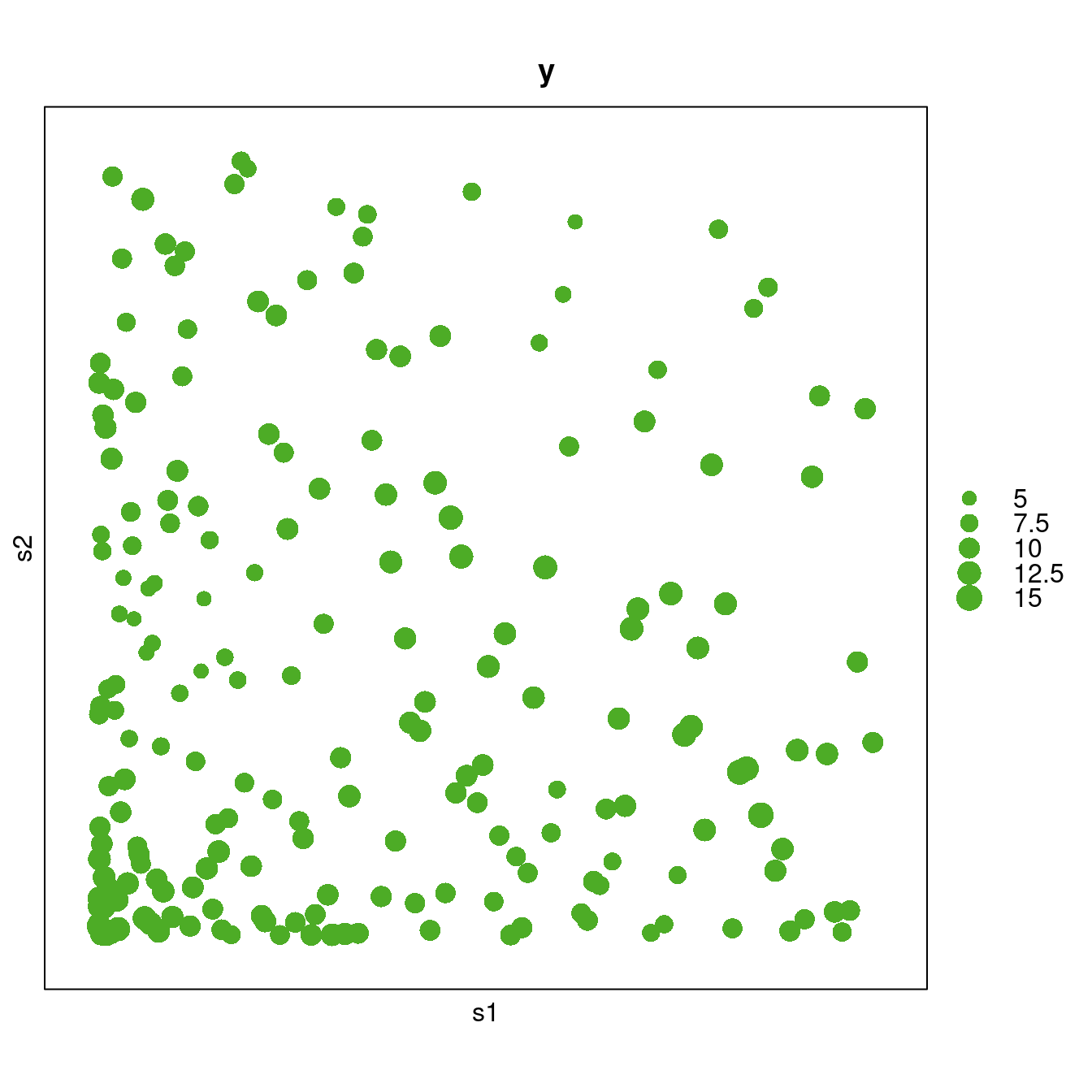

Figure 1.1: Bubble plot of the SPDEtoy dataset.

Figure 1.1 displays the values of the observations using a bubble plot. Here, a clear trend in the data can be observed, with more values observed close to the bottom left corner.

The first model we fit to the SPDEtoy dataset with INLA is a linear regression on the coordinates. This will be done using function inla(), which takes similar arguments to the lm(), glm() and gam() functions (to mention a few).
Under this model, observation \(y_i\) at location \(\mathbf{s}_i = (s_{1i}, s_{2i})\) is assumed to be distributed as a Gaussian variable with mean \(\mu_i\) and precision \(\tau\). The mean \(\mu_i\) is assumed to be equal to \(\alpha + \beta_1 s_{1i} + \beta_2 s_{2i}\), with \(\alpha\) the model intercept and \(\beta_1\) and \(\beta_2\) the coefficients of the covariates. By default, the prior on the intercept is a uniform distribution; the prior on the coefficients is also a Gaussian with zero mean and precision \(0.001\), and the prior on the precision \(\tau\) is a Gamma with parameters \(1\) and \(0.00005\). We can change the priors as discussed in Section 1.4.2.

We note that this example is used here simply to illustrate how to compute results with INLA. Furthermore, most of the models in this section are not reasonable spatial models since they lack rotation invariance of the coordinate system, which is a desirable property in many spatial models (see Chapter 2 for details).

The model can be stated as follows;

\[\begin{eqnarray} y_i & \sim & N(\mu_i, \tau^{-1}),\ i=1, \ldots,200 \nonumber \\ \mu_i & = & \alpha + \beta_1 s_{1i} + \beta_2 s_{2i} \nonumber \\ \alpha & \sim & \mbox{Uniform} \nonumber\\ \beta_j & \sim & N(0, 0.001^{-1}),\ j = 1,2 \nonumber\\ \tau & \sim & Ga(1, 0.00005). \nonumber\\ \end{eqnarray}\]

This linear model can be fitted as:

m0 <- inla(y ~ s1 + s2, data = SPDEtoy)

Although this is a simple example, there are many things going on behind the scenes. Default prior distributions on the intercept, the covariate coefficients, and the precision of the error term have been used. Secondly, the posterior marginals of the model parameters have been approximated using the INLA method and some quantities of interest (such as, for example, the marginal likelihood) have been computed.

A summary of the fitted model can be obtained as:

summary(m0)
## 
## Call:
##    "inla(formula = y ~ s1 + s2, data = SPDEtoy)" 
## Time used:
##     Pre = 0.456, Running = 0.0979, Post = 0.0256, Total = 0.58 
## Fixed effects:
##              mean   sd 0.025quant 0.5quant 0.975quant  mode
## (Intercept) 10.13 0.24      9.656    10.13      10.61 10.13
## s1           0.76 0.43     -0.081     0.76       1.61  0.76
## s2          -1.58 0.43     -2.428    -1.58      -0.74 -1.58
##             kld
## (Intercept)   0
## s1            0
## s2            0
## 
## Model hyperparameters:
##                                          mean    sd 0.025quant
## Precision for the Gaussian observations 0.308 0.031      0.251
##                                         0.5quant 0.975quant
## Precision for the Gaussian observations    0.307      0.372
##                                          mode
## Precision for the Gaussian observations 0.305
## 
## Expected number of effective parameters(stdev): 3.00(0.00)
## Number of equivalent replicates : 66.67 
## 
## Marginal log-Likelihood:  -423.18

The output provides a summary of the posterior marginals of the intercept, coefficients of the covariates and the precision of the error term. The posterior marginals of these parameters can be seen in Figure 1.2.

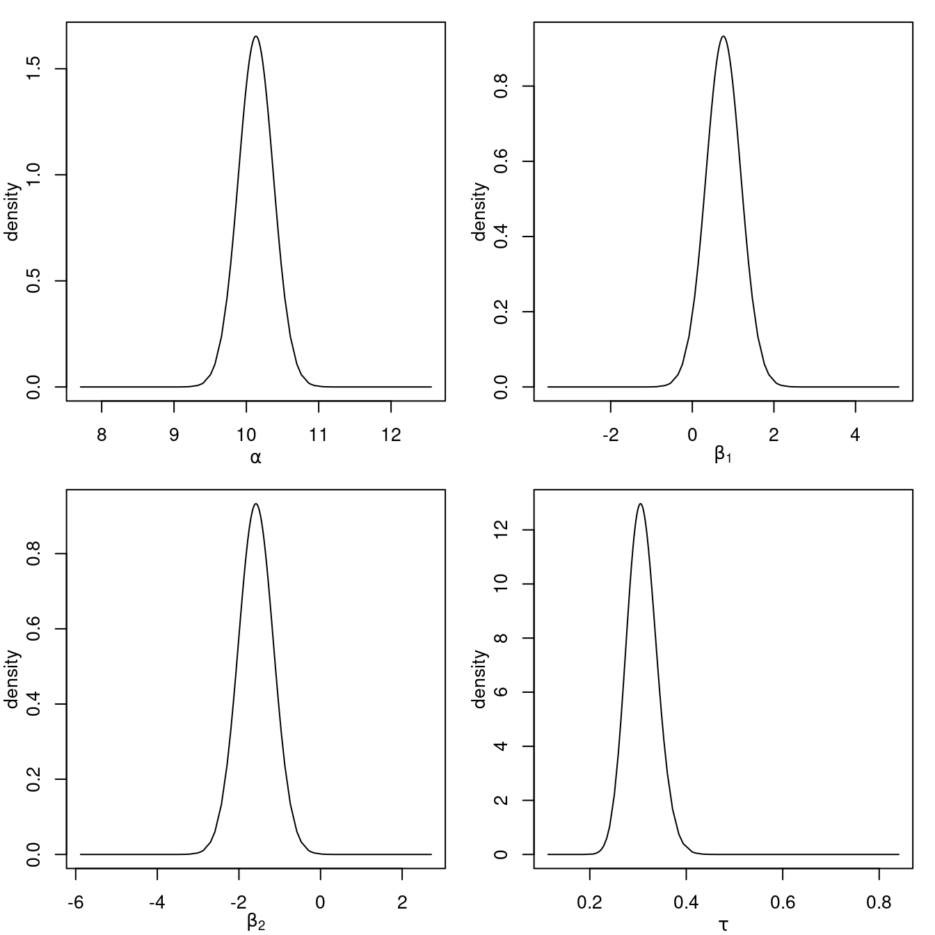
Figure 1.2: Posterior marginals of the parameters in the linear model fitted to the SPDEtoy dataset.

Note that the results provided in the summary of the model and the posterior marginals in Figure 1.2 both suggest that the value of the response decreases as the value of the y-coordinate s2 increases.

1.3.1 Non-linear effects of covariates

As described in Section 1.2, the INLA methodology can handle different types of effects, including random effects. In this case, in order to explore non-linear trends on the coordinates, a non-linear effect can be added on the covariates by using a random walk of order 1. This will replace the fixed effects on the covariates by a smooth term that may represent the effect of the coordinates better.

The vector of random effects \(\mathbf{u} = (u_1, \ldots, u_n)\) is defined assuming independent increments:

\[ \Delta u_i = u_i - u_{i+1} \sim N(0, \tau_{u}^{-1}), \ i = 1,\ldots, n - 1 \]

Here, \(\tau_u\) represents the precision of the random walk of order 1. Note that this is a discrete model and that, when it is defined on a continuous covariate (as in this case), the effect associated with observation \(y_i\) is \(u_{(i)}\). Here, the index \((i)\) is the position of the covariate associated with \(y_i\) used to define the model when all the values of the covariate are ordered increasingly.

Hence, the model now is defined using the following mean for the observations:

\[ \mu_i = \alpha + u_{1, (i)} + u_{2, (i')} \]

Vectors \(\mathbf{u}_1 = (u_{1,1}, \ldots, u_{1,n})\) and \(\mathbf{u}_2 = (u_{2,1}, \ldots, u_{2,n})\) represent the random effects associated with the covariates. Indices \((i)\) and \((i')\) are the positions of covariates \(s_{1i}\) and \(s_{2i}\), respectively. The precisions of the random effects are \(\tau_1\) and \(\tau_2\), respectively. By default, these parameters will be assigned a Gamma prior with parameters 1 and \(0.00005\). Full details about this model are available in the INLA package documentation, which can be viewed with inla.doc("rw1").

Random effects in INLA are defined by using the f() function within the formula that defines the model. The model defined before with non-linear terms on the covariates to introduce a smooth term on them can be fitted as:

f.rw1 <- y ~ f(s1, model = "rw1", scale.model = TRUE) +
  f(s2, model = "rw1", scale.model = TRUE)

In the previous formula, the f() function takes two arguments: the value of the covariate, and the type of random effect using the model argument. As we have decided to use a random walk of order one, the model is defined as model = "rw1". Furthermore, option scale.model = TRUE makes the model to be scaled to have an average variance of 1 (Sørbye and Rue 2014).

A complete list of implemented random effects can be obtained with inla.models()$latent. This will produce a named list with some computational details of the implemented models. A complete list with the names of the implemented models can be obtained with names(inla.models()$latent), or inla.list.models("latent").

Then, the model is fitted and summarized as follows:

m1 <- inla(f.rw1, data = SPDEtoy)

summary(m1)
## 
## Call:
##    "inla(formula = f.rw1, data = SPDEtoy)" 
## Time used:
##     Pre = 0.251, Running = 0.41, Post = 0.0327, Total = 0.694 
## Fixed effects:
##             mean   sd 0.025quant 0.5quant 0.97quant mode kld
## (Intercept)  9.9 0.12        9.6      9.9        10  9.9   0
## 
## Random effects:
##   Name     Model
##     s1 RW1 model
##    s2 RW1 model
## 
## Model hyperparameters:
##                                           mean     sd
## Precision for the Gaussian observations  0.352   0.04
## Precision for s1                         5.519  13.23
## Precision for s2                        41.329 152.94
##                                         0.025quant 0.5quant
## Precision for the Gaussian observations      0.279    0.351
## Precision for s1                             0.423    2.307
## Precision for s2                             1.330   12.201
##                                         0.97quant  mode
## Precision for the Gaussian observations     0.431 0.348
## Precision for s1                           27.152 0.882
## Precision for s2                          226.303 3.047
## 
## Expected number of effective parameters(stdev): 11.79(4.98)
## Number of equivalent replicates : 16.97 
## 
## Marginal log-Likelihood:  -1170.73

Figure 1.3 summarizes the effects fitted in this model. This includes the posterior marginals of the intercept \(\alpha\) and the precision of the error term \(\tau\), as well as the non-linear effects on the covariates. Note how the effect on the covariates is now slightly non-linear. The posterior marginals of the precisions of both random walks on covariates s1 and s2 (\(\tau_1\) and \(\tau_2\), respectively) have also been plotted.

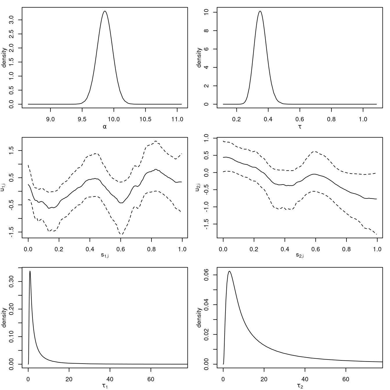
Figure 1.3: Posterior marginals of the intercept and precisions of the model with non-linear effects on the covariates fitted to the SPDEtoy dataset. The non-linear effects on the covariates are summarized using the posterior mean (solid line) and the limits of 95% credible intervals (dashed line).

The results show a decreasing trend on s2 but an unclear trend on s1. Furthermore, the posterior marginals of the precisions \(\tau_1\) and \(\tau_2\) show that the effect on covariate s2 has a stronger signal. Although this second model is more complex than the previous one it does not seem to improve model fitting, as the non-linear terms show no clear effect on s1 and a linear decreasing trend on s2. Note that the marginal likelihood cannot be used for the improper models, as the renormalization constant is not included. See inla.doc("rw1") for details.

1.3.2 inla objects

The object returned by function inla() is of type inla and it is a list that contains all the results from the model fitting with the INLA methodology. The actual results included may depend on the options used in the call to inla() (see Section 1.4 for some more details).

Table 1.2 describes some of the elements available in an inla object. Note that some of them are computed by default but that others (mostly the marginals of some effects and some model assessment criteria) are only computed when the appropriate options are passed on to inla().

Table 1.2: Elements in an inla object returned by a call to inla().

Function	Description
summary.fixed	Summary of fixed effects.
marginals.fixed	List of marginals of fixed effects.
summary.random	Summary of random effects.
marginals.random	List of marginals of random effects.
summary.hyperpar	Summary of hyperparameters.
marginals.hyperpar	List of marginals of the hyperparameters.
mlik	Marginal log-likelihood.
summary.linear.predictor	Summary of linear predictors.
marginals.linear.predictor	List of marginals of linear predictors.
summary.fitted.values	Summary of fitted values.
marginals.fitted.values	List of marginals of fitted values.

Summaries in an inla object are typically a data.frame with the estimates of the posterior mean, standard deviation, quantiles (by default, \(0.025\), \(0.5\) and \(0.975\)) and the mode. Marginals are represented in named lists by 2-column matrices, where the first column is the value of the parameter and the second column is the density.

For example, in order to display the summary of the fixed values from the linear regression model, we could do the following:

m0$summary.fixed
##               mean    sd 0.025quant 0.5quant 0.975quant   mode
## (Intercept) 10.132 0.242     9.6561   10.132      10.61 10.132
## s1           0.762 0.429    -0.0815    0.762       1.61  0.762
## s2          -1.584 0.429    -2.4276   -1.584      -0.74 -1.584
##                  kld
## (Intercept) 7.33e-07
## s1          7.33e-07
## s2          7.33e-07

For the fixed effects, inla() computes the symmetric Kullback-Leibler divergence using the Gaussian and Laplace approximations, and this is shown under column kld.

Similarly, the posterior marginal of the intercept \(\alpha\) could be plotted using:

plot(m0$marginals.fixed[[1]], type = "l", 
  xlab = expression(alpha), ylab = "density")

This is the command that has been used to produce the top-left plot in Figure 1.2. Marginals for the other fixed effects and hyperparameters could be plotted in a similar way. Calling plot() on an inla object will produce a number of default plots as well.

1.3.3 Prediction

Bayesian inference treats missing observations as any other parameter in the model (Little and Rubin 2002). When the missing observations are in the response variable, INLA automatically computes the predictive distribution of the corresponding linear predictor and fitted values. These missing observations in the response will be assigned the NA value in R, so that INLA knows that they are missing values.

In spatial statistics, prediction is often required when dealing with continuous spatial processes as the interest is in estimating the response variable at any point in the study region. In the next example, the predictive distribution of the response variable will be approximated at location (0.5, 0.5).

A new line to the SPDEtoy dataset will be added with the NA value and the coordinates of the point:

SPDEtoy.pred <- rbind(SPDEtoy, c(NA, 0.5, 0.5))

Next, the model will be fitted to the newly created SPDEtoy.pred dataset, which contains 201 observations. Note that option compute = TRUE needs to be set in control.predictor in order to compute the posterior marginals of the fitted values. The model with fixed effects on the covariates will be used:

m0.pred <- inla(y ~ s1 + s2, data = SPDEtoy.pred,
  control.predictor = list(compute = TRUE))

The results now provide the predictive distribution for the missing observation (in the 201st position of the list of marginals of the fitted values):

m0.pred$marginals.fitted.values[[201]]

This distribution is displayed in Figure 1.4. INLA provides several functions to manipulate the posterior marginals and compute quantities of interest, as explained in Section 1.5. For example, the posterior mean and variance could be easily computed.

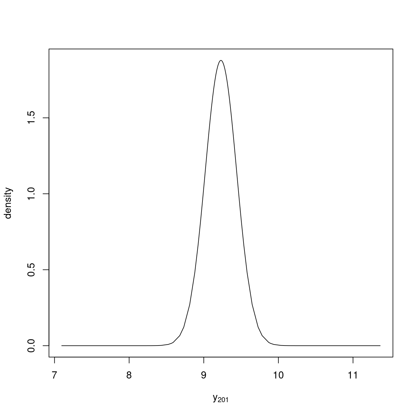
Figure 1.4: Predictive distribution of the response at location (0.5, 0.5).

1.4 Additional arguments and control options

As mentioned above, inla() can take a number of options that will help to define the model and the way the approximation with the INLA method is computed. Table 1.3 shows a few arguments that are sometimes required when defining a model. Some of them will be used in later sections of this book.

Table 1.3: Some arguments taken by inla() to define a model and produce a summary of model fitting.

Argument	Description
quantiles	Quantiles to be computed in the summary (default is c(0.025, 0.5, 0.975)).
E	Expected values (for some Poisson models, default is NULL).
offset	Offset to be added to the linear predictor (default is NULL).
weights	Weights on the observations (default is NULL)
Ntrials	Number of trials (for some binomial models, default is NULL).
verbose	Verbose output (default is FALSE).

Table 1.4 shows the main arguments taken by inla() to control the estimation process. Note that there are other control arguments not shown here.

Table 1.4: Some arguments taken by inla() to customize the estimation process.

Argument	Description
control.fixed	Control options for fixed effects.
control.family	Control options for the likelihood.
control.compute	Control options for what is computed (e.g., DIC, WAIC, etc.)
control.predictor	Control options for the linear predictor.
control.inla	Control options for how the posterior is computed.
control.results	Control options for computing the marginals of random effects and linear predictors.
control.mode	Control options to set the modes of the hyperparameters.

All the control arguments must take a named list with different options. These are conveniently described in the associated manual pages and will not be discussed here. For example, to find the list of possible options to be used with control.fixed, the user can type ?control.fixed in the R console.

A typical example of the use of these control options is computing some criteria for model selection and assessment, such as the DIC (Spiegelhalter et al. 2002), WAIC (Watanabe 2013), CPO (Pettit 1990), or PIT (Marshall and Spiegelhalter 2003). These can be computed by setting the appropriate options in control.compute:

m0.opts <- inla(y ~ s1 + s2, data = SPDEtoy,
  control.compute = list(dic = TRUE, cpo = TRUE, waic = TRUE)
)

The output with the new options is similar to the previous one, but now the DIC and the WAIC are reported:

summary(m0.opts)
## 
## Call:
##    c("inla(formula = y ~ s1 + s2, data = SPDEtoy, 
##    control.compute = list(dic = TRUE, ", " cpo = TRUE, 
##    waic = TRUE))") 
## Time used:
##     Pre = 0.188, Running = 0.245, Post = 0.0324, Total = 0.465 
## Fixed effects:
##              mean   sd 0.025quant 0.5quant 0.975quant  mode
## (Intercept) 10.13 0.24      9.656    10.13      10.61 10.13
## s1           0.76 0.43     -0.081     0.76       1.61  0.76
## s2          -1.58 0.43     -2.428    -1.58      -0.74 -1.58
##             kld
## (Intercept)   0
## s1            0
## s2            0
## 
## Model hyperparameters:
##                                          mean    sd 0.025quant
## Precision for the Gaussian observations 0.308 0.031      0.251
##                                         0.5quant 0.975quant
## Precision for the Gaussian observations    0.307      0.372
##                                          mode
## Precision for the Gaussian observations 0.305
## 
## Expected number of effective parameters(stdev): 3.00(0.00)
## Number of equivalent replicates : 66.67 
## 
## Deviance Information Criterion (DIC) ...............: 810.10
## Deviance Information Criterion (DIC, saturated) ....: 207.50
## Effective number of parameters .....................: 4.08
## 
## Watanabe-Akaike information criterion (WAIC) ...: 809.78
## Effective number of parameters .................: 3.69
## 
## Marginal log-Likelihood:  -423.18 
## CPO and PIT are computed
## 
## Posterior marginals for the linear predictor and
##  the fitted values are computed

The CPO and PIT are not reported, but a message in the output states that they have been computed. They can be accessed as:

m0.opts$cpo$cpo
m0.opts$cpo$pit

Figure 1.5 shows histograms of the computed CPO and PIT values for the model with fixed effects.

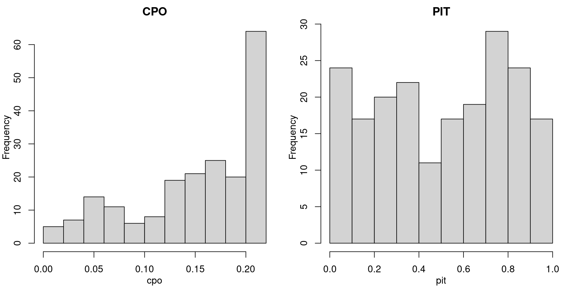
Figure 1.5: Histograms of CPO and PIT values for the model with fixed effects.

1.4.1 Estimation method

Other important options are related to the method used by INLA to approximate the posterior distribution of the hyperparameters. These are controlled by control.inla and some of them are summarized in Table 1.5.

The estimation method can be changed to achieve higher accuracy in the approximations or reduce the computation time by resorting to less accurate approximations. For example, the Gaussian approximation in INLA is less computationally expensive than the Laplace approximation.

Similarly, the integration strategy can be set in different ways. INLA uses a central composite design (CCD, Box and Draper 2007) to estimate the posterior distribution of the hyperparameters. This can be changed to an empirical Bayes (EB, Carlin and Louis 2008) strategy so that no integration of the hyperparameters is done. Other integration strategies are available, as listed in Table 1.5 and documented in the manual page of control.inla.

For example, we could compute the model with non-linear random effects using two different integration strategies and then compare the computation times. In particular, CCD and EB integration strategies will be compared:

m1.ccd <- inla(f.rw1, data = SPDEtoy,
  control.compute = list(dic = TRUE, cpo = TRUE, waic = TRUE),
  control.inla = list(int.strategy = "ccd"))
m1.eb <- inla(f.rw1, data = SPDEtoy,
  control.compute = list(dic = TRUE, cpo = TRUE, waic = TRUE),
  control.inla = list(int.strategy = "eb"))

Table 1.5: Some options that can be passed though control.inla to control the estimation process with INLA. Check the manual page (with ?control.inla) for more details.

Option	Description
strategy	Strategy used for the approximations: simplified.laplace (default), adaptive, gaussian or laplace.
int.strategy	Integration strategy: auto (default), ccd, grid or eb (check manual page for other options).

As seen below, the empirical Bayes integration strategy eb fits the model faster, but will likely provide less accurate approximations to the posterior marginals. In this example, the time difference is minimal, but for more complex models we can get massive speed-up from using eb.

# CCD strategy
m1.ccd$cpu.used
##     Pre Running    Post   Total 
## 0.23737 0.44166 0.03617 0.71520

# EB strategy
m1.eb$cpu.used
##     Pre Running    Post   Total 
## 0.22475 0.29174 0.03652 0.55300

1.4.2 Setting the priors

INLA has a set of predefined priors for all the effects in the model that will be used by default. However, prior specification is a key step in Bayesian analysis and careful attention should be paid to the specification of the priors in the model.

For the fixed effects, the default prior is a Gaussian distribution with zero mean, and the precision is zero for the intercept and \(0.001\) for the coefficients of the covariates. These values for the Gaussian prior can be changed with argument control.fixed using the variables listed in Figure 1.6. More information is available in the manual page (which can be accessed with ?control.fixed).

Table 1.6: Options to set the prior of the fixed effects in argument control.fixed.

Option	Description
mean.intercept	Prior mean for the intercept (default is \(0\)).
prec.intercept	Prior precision for the intercept (default is \(0\)).
mean	Prior mean for the coefficients of the covariates (default is \(0\)). It can be a named list.
prec	Prior precision for the coefficients of the covariates (default is \(0.001\)). It can be a named list.

The parameters in the likelihood can also be assigned a prior by means of variable hyper in argument control.likelihood. Similarly, the hyperparameters of the random effects defined through the f() function can be assigned a prior using argument hyper. In both cases, hyper will be a named list (using the names of the hyperparameters) and each value will be a list with the options listed in Table 1.7.

Table 1.7: Options to set the prior of the hyperparameters in the likelihood and random effects.

Option	Description
initial	Initial value of the hyperparameter.
prior	Prior distribution to be used.
param	Vector with the values of the parameters of the prior distribution.
fixed	Boolean variable to set the parameter to a fixed value (default FALSE).

In order to show how the different priors are defined, we will fit the model with non-linear effects again. Note that all priors are set in the internal scale of the parameters in INLA. This is reported in the package documentation and, for example, the precision is represented internally in the log-scale, so that the prior is set on the log-precision.

First of all, fixed effects will be set to have a Gaussian prior with zero mean and precision 1. These are the options that will be passed using argument control.fixed:

# Prior on the fixed effects
prior.fixed <- list(mean.intercept = 0, prec.intercept = 1,
  mean = 0, prec = 1)

Similarly, the log-precision in the Gaussian likelihood of the model will be assigned a Gaussian prior with zero mean and precision 1, and this will be passed using argument control.family:

# Prior on the likelihood precision (log-scale)
prior.prec <- list(initial = 0, prior = "normal", param = c(0, 1),
  fixed = FALSE)

Note how the initial value is set to zero as it is in the internal scale; i.e., the initial value of the precision is \(\exp(0) = 1\).

Finally, the precision of the random walks will be fixed to \(1\) (i.e., \(0\) in the internal scale):

# Prior on the precision of the RW1
prior.rw1 <- list(initial = 0, fixed = TRUE)

This means that the hyperparameter is not estimated but fixed to the value provided and, hence, it will not be reported in the output.

The following R code shows the call to fit the model using the different sets of priors. Note how the priors on the likelihood hyperparameters and the random effects need to be embedded in a named list using the name of the hyperparameter:

f.hyper <- y ~ 1 +
  f(s1, model = "rw1", hyper = list(prec = prior.rw1),
    scale.model = TRUE) +
  f(s2, model = "rw1", hyper = list(prec = prior.rw1),
    scale.model = TRUE)

m1.hyper <- inla(f.hyper, data = SPDEtoy,
  control.fixed = prior.fixed,
  control.family = list(hyper = list(prec = prior.prec)))

A summary of the model can be obtained as follows:

summary(m1.hyper)
## 
## Call:
##    c("inla(formula = f.hyper, data = SPDEtoy, 
##    control.family = list(hyper = list(prec = prior.prec)), 
##    ", " control.fixed = prior.fixed)") 
## Time used:
##     Pre = 0.226, Running = 0.158, Post = 0.0314, Total = 0.415 
## Fixed effects:
##              mean    sd 0.025quant 0.5quant 0.975quant  mode
## (Intercept) 9.726 0.117      9.494    9.726      9.953 9.728
##             kld
## (Intercept)   0
## 
## Random effects:
##   Name     Model
##     s1 RW1 model
##    s2 RW1 model
## 
## Model hyperparameters:
##                                         mean    sd 0.025quant
## Precision for the Gaussian observations 0.37 0.039      0.297
##                                         0.5quant 0.975quant
## Precision for the Gaussian observations    0.368      0.452
##                                          mode
## Precision for the Gaussian observations 0.365
## 
## Expected number of effective parameters(stdev): 20.41(1.07)
## Number of equivalent replicates : 9.80 
## 
## Marginal log-Likelihood:  -1194.30

As mentioned above, the precisions of the non-linear terms on the covariates are not reported because they have been fixed to 1.

A complete list of the priors available in the INLA package (and their options) can be obtained with inla.models()$prior. This is a named list, and the names of the priors can be easily checked with names(inla.models()$prior). These are also described in the R-INLA package documentation. An alternative, is to use inla.list.models("prior"). Additionally, there is an option for user defined priors through tables or R expressions.

1.5 Manipulating the posterior marginals

The INLA package comes with a number of functions to manipulate the posterior marginals returned by the inla() function. These are summarized in Table 1.8 and specific information can be found in their respective manual pages.

Table 1.8: Functions to manipulate the posterior marginals.

Function	Description
inla.emarginal()	Compute the expectation of a function.
inla.dmarginal()	Compute the density.
inla.pmarginal()	Compute a probability.
inla.qmarginal()	Compute a quantile.
inla.rmarginal()	Sample from the marginal.
inla.hpdmarginal()	Compute a high probability density (HPD) interval.
inla.smarginal()	Interpolate the posterior marginal.
inla.mmarginal()	Compute the mode.
inla.tmarginal()	Transform the marginal.
inla.zmarginal()	Compute summary statistics.

A typical example of the use of these functions is to compute the posterior marginal of the variance of the error term (i.e., \(1/\tau\)). This would involve a transformation of the posterior marginal on \(\tau\), and then computing some summary statistics.

The transformation can be done using function inla.tmarginal(), which will take the function for the transformation and the marginal. We strongly recommend transforming the internal.marginals.hyperpar instead of the marginals.hyperpar. The internal.marginals.hyperpar reports the marginals of the hyperparameters in the internal scale, like \(\log(\tau)\) in this example:

# Compute posterior marginal of variance
post.var <- inla.tmarginal(function(x) exp(-x), 
  m0$internal.marginals.hyperpar[[1]])

Summary statistics can be computed with function inla.zmarginal():

# Compute summary statistics
inla.zmarginal(post.var)
## Mean            3.27667 
## Stdev           0.329572 
## Quantile  0.025 2.692 
## Quantile  0.25  3.04381 
## Quantile  0.5   3.25437 
## Quantile  0.75  3.48478 
## Quantile  0.975 3.98491

Similarly, a 95% high probability interval (HPD) can be computed as:

inla.hpdmarginal(0.95, post.var)
##              low  high
## level:0.95 2.655 3.936

1.6 Advanced features

In this section we will describe some advanced features available in the INLA package for model fitting. In particular, the use of the models with more than one likelihood, how to define models that share effects between different parts of the model, how to create linear combinations on the latent effects and the use of Penalized Complexity priors. More details about advanced features can be found in the R-INLA website at http://www.r-inla.org/models/tools.

1.6.1 Several likelihoods

INLA can handle models with more than one likelihood. This is a common modeling approach to build joint models. For example, in survival analysis survival times may be related to some outcome of interest that may be modeled jointly using a longitudinal model (Ibrahim, Chen, and Sinha 2001). By using a model with more than one likelihood it is possible to build a joint model with different types of outputs and the hyperparameters in the likelihoods will be fitted separately.

In order to provide a simple example, we will consider a similar toy dataset to the SPDEtoy one with added noise. This would mimic a situation in which two sets of measurements are available but with different noise effects. This new dataset can be created by adding random Gaussian noise (with standard deviation equal to 2) to the original observations in the SPDEtoy dataset:

library(INLA)
data(SPDEtoy)
SPDEtoy$y2 <- SPDEtoy$y + rnorm(nrow(SPDEtoy), sd = 2)

Hence, both sets of observations can be modeled on the same covariates but the precisions of the error terms are different, and these should be modeled separately. A simple way to do this is to fit a model with two Gaussian likelihoods with different precisions to be estimated by each one of the sets of observations.

The model that will be fitted is the following:

\[\begin{eqnarray} y_i & \sim & N(\mu_i, \tau_1^{-1}),\ i = 1,\ldots, 200 \nonumber \\ y_i & \sim & N(\mu_i, \tau_2^{-1}),\ i = 201,\ldots, 400 \nonumber \\ \mu_i & = & \alpha + \beta_1 s_{1i} + \beta_2 s_{2i},\ i=1,\ldots,400 \nonumber \\ \alpha & \sim & \mbox{Uniform} \nonumber\\ \beta_j & \sim & N(0, 0.001^{-1}),\ j = 1, 2 \nonumber\\ \tau_j & \sim & Ga(1, 0.00005),\ j = 1, 2 \nonumber\\ \end{eqnarray}\]

In order to fit a model with more than one likelihood the response variable must be a matrix with as many columns as the number of likelihoods. The number of rows is the total number of observations. Given a column, the rows with data not associated with that likelihood are filled with NA values. In our example, this can be done as follows:

# Number of locations
n <- nrow(SPDEtoy)

# Response matrix
Y <- matrix(NA, ncol = 2, nrow = n * 2)

# Add `y` in first column, rows 1 to 200
Y[1:n, 1] <- SPDEtoy$y
# Add `y2` in second column, rows 201 to 400
Y[n + 1:n, 2] <- SPDEtoy$y2

Note how the values of y are added in the first column in rows 1 to n, and the values of y2 are added to the second column in rows from n + 1 to 2 * n, where n is the number of locations in the SPDEtoy dataset.

Using more than one likelihood may affect other elements in the model definition, such as if the model incorporates in the likelihood some of the values described in Table 1.3.

The covariates will be the same in both likelihoods, so they do not need to be modified in any way. The family argument must be a vector with the names of the likelihoods used. In this case, it will be family = c("gaussian", "gaussian") but different likelihoods can be used.

Then, the model can be fitted as follows:

m0.2lik <- inla(Y ~ s1 + s2, family = c("gaussian", "gaussian"),
  data = data.frame(Y = Y,
    s1 = rep(SPDEtoy$s1, 2),
    s2 = rep(SPDEtoy$s2, 2))
)

The summary of this model now shows estimates of two precisions:

summary(m0.2lik)
## 
## Call:
##    c("inla(formula = Y ~ s1 + s2, family = c(\"gaussian\", 
##    \"gaussian\"), ", " data = data.frame(Y = Y, s1 = 
##    rep(SPDEtoy$s1, 2), s2 = rep(SPDEtoy$s2, ", " 2)))") 
## Time used:
##     Pre = 0.465, Running = 0.262, Post = 0.027, Total = 0.755 
## Fixed effects:
##               mean    sd 0.025quant 0.5quant 0.975quant   mode
## (Intercept) 10.219 0.203      9.820   10.219     10.618 10.218
## s1           0.571 0.360     -0.138    0.571      1.278  0.572
## s2          -1.642 0.360     -2.349   -1.642     -0.936 -1.642
##             kld
## (Intercept)   0
## s1            0
## s2            0
## 
## Model hyperparameters:
##                                             mean    sd
## Precision for the Gaussian observations    0.309 0.031
## Precision for the Gaussian observations[2] 0.128 0.013
##                                            0.025quant 0.5quant
## Precision for the Gaussian observations         0.252    0.308
## Precision for the Gaussian observations[2]      0.104    0.127
##                                            0.975quant  mode
## Precision for the Gaussian observations         0.374 0.306
## Precision for the Gaussian observations[2]      0.154 0.127
## 
## Expected number of effective parameters(stdev): 3.00(0.00)
## Number of equivalent replicates : 133.32 
## 
## Marginal log-Likelihood:  -927.21

Note how the precision of the second likelihood has a posterior mean smaller to the precision of the first likelihood. This is because the variance of the second set of observations is higher as they were generated by adding some noise to the original data. Also, the estimates of the fixed effects are very similar to the ones estimated in the previous models.

1.6.2 Copy model

Sometimes it is necessary to share an effect that is estimated from two or more parts of the dataset, so that all of them provide information about the effect when fitting the model. This is known as a copy effect, as the new effect will be a copy of the original effect plus some tiny noise.

To illustrate the use of the copy effect in INLA we will fit a model where the fixed effect of the y-coordinate is copied. In particular, this will be the fitted model:

\[\begin{eqnarray} y_i & \sim & N(\mu_i, \tau^{-1}),\ i = 1,\ldots, 400 \nonumber \\ \mu_i & = & \alpha + \beta_1 s_{1i} + \beta_2 s_{2i},\ i=1,\ldots,200 \nonumber \\ \mu_i & = & \alpha + \beta_1 s_{1i} + \beta \cdot\beta^{*}_2 s_{2i},\ i=201,\ldots,400 \nonumber \\ \alpha & \sim & \mbox{Uniform} \nonumber\\ \beta_j & \sim & N(0, 0.001^{-1}),\ j = 1, 2 \nonumber\\ \beta^*_2 & \sim & N(\beta_2, \tau_{\beta_2}^{-1} = 1 / \exp(14)) \nonumber \\ \tau_j & \sim & Ga(1, 0.00005),\ j = 1, 2 \nonumber \end{eqnarray}\]

Here, \(\beta^*_2\) is the copied effect (from \(\beta_2\)). Note how the copied effect has a scaling factor, \(\beta\), but this is fixed to 1 by default. Furthermore, the precision of \(\beta_2^*\) is set to a very large value, ensuring that the copied effect is very close to \(\beta_2\). This precision can be set using argument precision in the call of the f() function (see below).

Before implementing the model in INLA, a new data.frame with the original SPDEtoy data and the simulated one will be put together. This will involve creating two new vectors of covariates by repeating the original covariates. Furthermore, two indices will be created to identify to which group of observations a value belongs:

y.vec <- c(SPDEtoy$y, SPDEtoy$y2)
r <- rep(1:2, each = nrow(SPDEtoy))
s1.vec <- rep(SPDEtoy$s1, 2)
s2.vec <- rep(SPDEtoy$s2, 2)
i1 <- c(rep(1, n), rep(NA, n))
i2 <- c(rep(NA, n), rep(1, n))

d <- data.frame(y.vec, s1.vec, s2.vec, i1, i2)

The copied effect will be defined using independent and identically distributed random effects with a single group that will be multiplied by the values of the covariates. This is an alternative way to define a linear effect in INLA in a way that allows the effect to be copied. This model is implemented as the iid model in INLA. See inla.doc("iid") for details.

For this reason, indices i1 and i2 have either 1 (i.e., the linear predictor includes the random effect) or NA (there is no random effect in the linear predictor). This ensures that the linear predictor includes the original random effect in the first 200 observations (using index i1), and the copied effect in the last 200 observations (using index i2).

Given that the model is now implemented using a single random effect with the covariate values as weights, the precision of the random effect needs to be fixed to 0.001 in order to obtain similar results as in previous models. This can be done by using an initial value for the precision of the random effects and fixing it in the prior definition. The values to be passed to the prior definition (in the call to the f() function below) are:

tau.prior = list(prec = list(initial = 0.001, fixed = TRUE))

Then, the formula to fit the model is defined using first an iid model with an index i1 which is 1 for the first n values and NA for the rest. The copied effect uses an index for the second set of observations, and the values of the covariates as weights:

f.copy <- y.vec ~ s1.vec + 
  f(i1, s2.vec, model = "iid", hyper = tau.prior) +
  f(i2, s2.vec, copy = "i1")

Finally, the model is fitted and summarized as:

m0.copy <- inla(f.copy, data = d)

summary(m0.copy)
## 
## Call:
##    "inla(formula = f.copy, data = d)" 
## Time used:
##     Pre = 0.449, Running = 0.158, Post = 0.0197, Total = 0.627 
## Fixed effects:
##               mean    sd 0.025quant 0.5quant 0.975quant   mode
## (Intercept) 10.201 0.218      9.772   10.201     10.629 10.202
## s1.vec       0.444 0.397     -0.336    0.444      1.222  0.444
##             kld
## (Intercept)   0
## s1.vec        0
## 
## Random effects:
##   Name     Model
##     i1 IID model
##    i2 Copy
## 
## Model hyperparameters:
##                                         mean    sd 0.025quant
## Precision for the Gaussian observations 0.18 0.013      0.156
##                                         0.5quant 0.975quant
## Precision for the Gaussian observations    0.179      0.206
##                                          mode
## Precision for the Gaussian observations 0.179
## 
## Expected number of effective parameters(stdev): 2.86(0.009)
## Number of equivalent replicates : 139.66 
## 
## Marginal log-Likelihood:  -931.41

Note that with this particular parameterization of the model, the coefficient of s2 is in fact a random effect and that it is available in the summary of the random effects:

m0.copy$summary.random
## $i1
##   ID  mean    sd 0.025quant 0.5quant 0.975quant  mode      kld
## 1  1 -1.45 0.369      -2.18    -1.45     -0.729 -1.46 1.48e-07
## 
## $i2
##   ID  mean    sd 0.025quant 0.5quant 0.975quant  mode      kld
## 1  1 -1.45 0.369      -2.18    -1.45     -0.729 -1.46 1.48e-07

Alternatively, the copied effect can also be multiplied by a scaling factor \(\beta\), which is estimated. This can be achieved by adding fixed = FALSE to the definition of the copied effect:

f.copy2 <- y.vec ~ s1.vec + f(i1, s2.vec, model = "iid") +
  f(i2, s2.vec, copy = "i1", fixed = FALSE)

In this case, the estimate of this coefficient should be close to one as the copied effect is exactly the same for the second group of observations:

m0.copy2 <- inla(f.copy2, data = d)
summary(m0.copy2)
## 
## Call:
##    "inla(formula = f.copy2, data = d)" 
## Time used:
##     Pre = 0.285, Running = 0.266, Post = 0.0286, Total = 0.579 
## Fixed effects:
##              mean    sd 0.025quant 0.5quant 0.975quant  mode
## (Intercept) 9.701 0.181      9.346    9.701     10.056 9.701
## s1.vec      0.491 0.405     -0.304    0.491      1.285 0.491
##             kld
## (Intercept)   0
## s1.vec        0
## 
## Random effects:
##   Name     Model
##     i1 IID model
##    i2 Copy
## 
## Model hyperparameters:
##                                             mean       sd
## Precision for the Gaussian observations 1.72e-01 1.20e-02
## Precision for i1                        1.83e+04 1.82e+04
## Beta for i2                             1.00e+00 3.16e-01
##                                         0.025quant 0.5quant
## Precision for the Gaussian observations      0.149 1.72e-01
## Precision for i1                          1232.029 1.29e+04
## Beta for i2                                  0.379 1.00e+00
##                                         0.975quant     mode
## Precision for the Gaussian observations   1.98e-01    0.171
## Precision for i1                          6.66e+04 3348.244
## Beta for i2                               1.62e+00    1.001
## 
## Expected number of effective parameters(stdev): 2.00(0.001)
## Number of equivalent replicates : 199.90 
## 
## Marginal log-Likelihood:  -938.12

In the previous output, Beta for i2 refers to the scaling coefficient \(\beta\) that multiplies the copied effect. It can be seen how its posterior mean is very close to one, as expected.

1.6.3 Replicate model

The copy effect described in the previous section is useful to create an effect which is very close to the copied one. The replicate effect in INLA is similar to the copy effect but, in this case, the values of the hyperparameters will be shared by the different replicated effects. This means that, for example, if an iid effect is replicated, the replicated random effects will be independent with the same precision.

To show the use of the replicate feature in INLA a linear latent model will be used. The coefficients will be replicated considered the first half of the observations in one group and the second half of the observations in the secod. Coefficients will be modeled using an iid random effect with a precision fixed to \(0.001\) and the values of the covariates as weights. This is essentially an alternative implementation of a linear fixed effect that can be defined through the f() function. Note that although the linear latent effect can be used to define linear effects, it does not allow for replication.

The linear effects will be replicated for both covariates s1 and s2. By replicating this effect, the same precision is used in the prior of all the replicated coefficients. Each covariate will have two replicated coefficients, each one estimated half the data. Although in this example the precision is fixed (to mimick how fixed effects are defined in INLA), it is possible to assign a prior to the precision, having an extra level in the hierarchical model.

The index to create the replicated effects is created by defining a vector with two values as follows:

d$r <- rep(1:2, each = nrow(SPDEtoy))

Index r defines how the observations are grouped to estimate the replicated effects. In this case, the first 200 observations are in the first group and the last 200 in the second group.

As we are defining the replicated effects on two covariates, two additional indices are required. These indices will have an unique value (1, in this case) because the grouping of the observations into two groups will be done with the replication index (i.e., r). Note that this is naïve example to show how replicated effects work and that the random effects indices could well define the two different groups.

Hence, the indices to define the linear effects using the iid latent effects are:

d$idx1 <- 1
d$idx2 <- 1

Then, the linear effects can be replicated in the formula that defines the model as:

f.rep <- y.vec ~ 1 + 
  f(idx1, s1.vec, model = "iid", replicate = r, hyper = tau.prior) +
  f(idx2, s2.vec, model = "iid", replicate = r, hyper = tau.prior)

Note that the hyper argument is used to fix the precision of the iid effects to \(0.001\).

Finally, the model with the replicated effects can be easily fitted:

m0.rep <- inla(f.rep, data = d)

summary(m0.rep)
## 
## Call:
##    "inla(formula = f.rep, data = d)" 
## Time used:
##     Pre = 0.273, Running = 0.162, Post = 0.0196, Total = 0.455 
## Fixed effects:
##              mean    sd 0.025quant 0.5quant 0.975quant  mode
## (Intercept) 10.18 0.203      9.778    10.18      10.58 10.18
##             kld
## (Intercept)   0
## 
## Random effects:
##   Name     Model
##     idx1 IID model
##    idx2 IID model
## 
## Model hyperparameters:
##                                          mean    sd 0.025quant
## Precision for the Gaussian observations 0.179 0.013      0.155
##                                         0.5quant 0.975quant
## Precision for the Gaussian observations    0.179      0.205
##                                          mode
## Precision for the Gaussian observations 0.178
## 
## Expected number of effective parameters(stdev): 4.20(0.046)
## Number of equivalent replicates : 95.20 
## 
## Marginal log-Likelihood:  -930.40

The summary of the estimated coefficients are part of the random effects and they can be shown as follows:

m0.rep$summary.random
## $idx1
##   ID   mean     sd 0.025quant 0.5quant 0.975quant   mode
## 1  1 0.4769 0.4465    -0.4006   0.4771      1.353 0.4775
## 2  1 0.2059 0.4465    -0.6713   0.2060      1.082 0.2062
##         kld
## 1 1.313e-07
## 2 1.136e-07
## 
## $idx2
##   ID   mean     sd 0.025quant 0.5quant 0.975quant   mode
## 1  1 -1.320 0.4471     -2.196   -1.320    -0.4409 -1.322
## 2  1 -1.243 0.4469     -2.119   -1.244    -0.3647 -1.245
##         kld
## 1 3.643e-07
## 2 3.139e-07

The replicated coefficients for each covariate look similar as the actual effect is the same but not exactly equal because each one is estimated using half the observations.

Finally, note how the summaries of the effects and hyperparameters are very similar to those obtained in previous examples.

1.6.4 Linear combinations of the latent effects

INLA can also handle models in which the linear predictors defined in the model formula are multiplied by a matrix A (called the observation matrix in the package documentation). This is, the vector of linear predictors on the fixed and random effects \(\boldeta\) defined by the model formula becomes

\[ {\boldeta^*}^{\top} = A \boldeta^{\top} \]

Here, \(\boldeta^*\) is the actual linear predictor used when fitting the model and it is a linear combination of the effects in \(\boldeta\). Note that \(\boldeta\) is the linear predictor as defined by the model formula passed to inla().

In order to provide a simple example, we define A as a diagonal matrix with values of 10 in the diagonal. This is similar to multiplying all the effects in the linear predictor by 10, which will make the estimates of the intercept and the covariate coefficients shrink by a factor of 10. This is done as follows:

# Define A matrix
A = Diagonal(n + n, 10)

# Fit model
m0.A <- inla(f.rep, data = d, control.predictor = list(A = A))

The summary of the fitted model can be seen below. Note how the estimates of the fixed effects are shrunk by a factor of 10 but that the estimate of the precision does not change. This is because the A matrix only affects the linear predictor and not the error term.

summary(m0.A)
## 
## Call:
##    "inla(formula = f.rep, data = d, control.predictor = 
##    list(A = A))" 
## Time used:
##     Pre = 0.311, Running = 0.159, Post = 0.0186, Total = 0.489 
## Fixed effects:
##              mean    sd 0.025quant 0.5quant 0.975quant  mode
## (Intercept) 1.028 0.022      0.984    1.028      1.072 1.028
##             kld
## (Intercept)   0
## 
## Random effects:
##   Name     Model
##     idx1 IID model
##    idx2 IID model
## 
## Model hyperparameters:
##                                          mean    sd 0.025quant
## Precision for the Gaussian observations 0.179 0.013      0.155
##                                         0.5quant 0.975quant
## Precision for the Gaussian observations    0.179      0.205
##                                          mode
## Precision for the Gaussian observations 0.178
## 
## Expected number of effective parameters(stdev): 5.03(0.004)
## Number of equivalent replicates : 79.47 
## 
## Marginal log-Likelihood:  -939.16

Although this is a very simple example, the A matrix can be useful when the linear predictors in \(\boldeta\) need to be linearly combined to define more complex linear predictors, such as to allow the effects of the covariates of one observation to influence other observations.

The use of the A matrix plays an important role in the spatial models described through this book. In particular, the A matrix allows us to include linear combinations of some random effects in the model that are needed to define some spatial models. Given the complexity of manually constructing an A matrix from the different effects, we will use helper functions like inla.stack() to create this matrix.

1.6.5 Penalized Complexity priors

Simpson et al. (2017) describe a new approach for constructing prior distributions called Penalized Complexity priors, or PC priors for short. Under this new framework, a PC prior for the standard deviation \(\sigma\) of a latent effect is set by defining parameters \((u, \alpha)\) so that

\[ \textrm{Prob}(\sigma > u) = \alpha,\ u > 0,\ 0 < \alpha < 1. \]

Hence, PC priors provide a different way to propose priors on the model hyperparameters.

Section 1.3.1 shows an example of fitting a model with two random walks of order one on s1 and s2 with default Gamma priors on the precision parameters. To set a PC prior on the standard deviation of the random walk, we consider the complexity of the latent effect; e.g., for this effect we believe that the probability of the standard deviation being higher than 1 is quite small. Hence, we set \(u = 1\) and \(\alpha = 0.01\).

The PC-prior on the standard deviation of the random walk latent effect is then defined as:

pcprior <- list(prec = list(prior = "pc.prec",
  param = c(1, 0.01)))

This definition will be passed to the f() function when the latent effect is defined in the model formula:

f.rw1.pc <- y ~ 
  f(s1, model = "rw1", scale.model = TRUE, hyper = pcprior) +
  f(s2, model = "rw1", scale.model = TRUE, hyper = pcprior)

Next, the model is fitted and the resulting estimates shown:

m1.pc <- inla(f.rw1.pc, data = SPDEtoy)

summary(m1.pc)
## 
## Call:
##    "inla(formula = f.rw1.pc, data = SPDEtoy)" 
## Time used:
##     Pre = 0.225, Running = 0.335, Post = 0.0269, Total = 0.587 
## Fixed effects:
##              mean    sd 0.025quant 0.5quant 0.975quant  mode
## (Intercept) 9.858 0.119      9.623    9.858      10.09 9.858
##             kld
## (Intercept)   0
## 
## Random effects:
##   Name     Model
##     s1 RW1 model
##    s2 RW1 model
## 
## Model hyperparameters:
##                                          mean     sd
## Precision for the Gaussian observations 0.356  0.039
## Precision for s1                        3.650  4.599
## Precision for s2                        8.105 11.200
##                                         0.025quant 0.5quant
## Precision for the Gaussian observations      0.283    0.355
## Precision for s1                             0.588    2.274
## Precision for s2                             1.138    4.802
##                                         0.975quant  mode
## Precision for the Gaussian observations      0.437 0.353
## Precision for s1                            15.088 1.202
## Precision for s2                            35.413 2.397
## 
## Expected number of effective parameters(stdev): 13.19(3.79)
## Number of equivalent replicates : 15.16 
## 
## Marginal log-Likelihood:  -1158.64

The estimates of the intercept and the precision of the Gaussian likelihood are very similar to the model fitted in Section 1.3.1. The estimates of the precisions of the random walks associated with s1 and s2 seem to be different. In particular, the precision of the random walk on s2 is certainly smaller than when default Gamma priors are used.

In order to inspect the effect of the PC prior we have computed the posterior marginals of the standard deviations of both random walks:

post.sigma.s1 <- inla.tmarginal(function (x) sqrt(1 / exp(x)),
  m1.pc$internal.marginals.hyperpar[[2]])

post.sigma.s2 <- inla.tmarginal(function (x) sqrt(1 / exp(x)),
  m1.pc$internal.marginals.hyperpar[[3]])

Figure 1.6 shows the posterior marginals of the standard deviations. The PC prior makes the posterior have most of its density below one. In this particular case there are some differences between using a default Gamma prior and a PC prior with parameters \((1, 0.01)\).

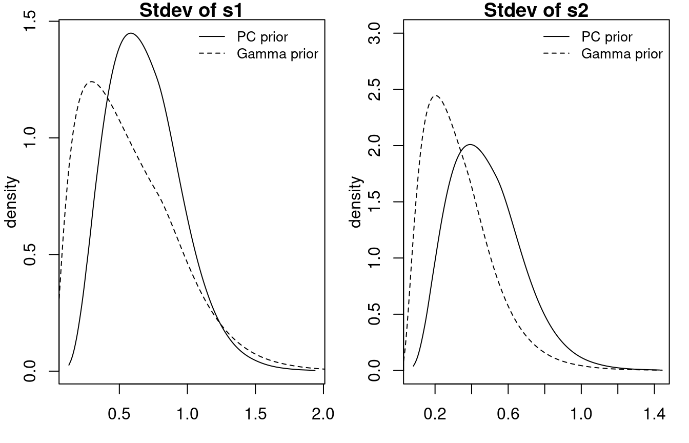
Figure 1.6: Posterior marginals of the standard deviations of two random walks using a PC prior and the default Gamma prior.

More information about the PC prior used in this example can be found in the manual page that can be accessed by typing inla.doc("pc.prec") in R. Other PC priors will be introduced later in the book to propose priors for other types of spatial latent effects.

Section 2.8.2.2 shows the use of PC priors in a spatial model. In this case, the relevant parameters are the standard deviation of the spatial process and the range, which measures a distance at which spatial autocorrelation is small. PC priors in this case are defined using the same principle as above for both parameters. For the standard deviation \(\sigma\) we need to define \((\sigma_0, \alpha)\) so that

\[ P(\sigma > \sigma_0) = \alpha, \]

while for the range \(r\) we need to define \((r_0, \alpha)\) so that

\[ P(r < r_0) = \alpha. \]

References

Bakka, H., H. Rue, G.-A. Fuglstad, A. Riebler, D. Bolin, E. Krainski, D. Simpson, and F. Lindgren. 2018. “Spatial Modelling with R-INLA: A Review.” WIREs Comput Stat 10 (6): 1–24. https://doi.org/10.1002/wics.1443.

Bivand, R. S., E. J. Pebesma, and V. Gomez-Rubio. 2013. Applied Spatial Data Analysis with R. 2nd ed. Springer, NY. http://www.asdar-book.org/.

Blangiardo, M., and M. Cameletti. 2015. Spatial and SpatioTemporal Bayesian Models with R-INLA. Chichester, UK: John Wiley & Sons, Ltd.

Box, G. E., and N. R. Draper. 2007. Response Surfaces, Mixtures, and Ridge Analyses. 2nd ed. Hoboken, NJ: Wiley-Interscience.

Carlin, B. P., and T. A. Louis. 2008. Bayesian Methods for Data Analysis. 3rd ed. Boca Raton, FL: Chapman & Hall/CRC.

Gilks, W. R., S. Richardson, and D. J. Spiegelhalter. 1996. Markov Chain Monte Carlo in Practice. Boca Raton, FL: Chapman & Hall.

Gómez-Rubio, V. 2019. Bayesian Inference with INLA. Chapman & Hall/CRC.

Ibrahim, J. G., M-H. Chen, and D. Sinha. 2001. Bayesian Survival Analysis. New York: Springer-Verlag.

Little, R. J. A., and D. B. Rubin. 2002. Statistical Analysis with Missing Data. 2nd ed. Hoboken, NJ: John Wiley; Sons.

Marshall, E. C., and D. J. Spiegelhalter. 2003. “Approximate Cross-Validatory Predictive Checks in Disease Mapping Models.” Statistics in Medicine 22 (10): 1649–60.

Pettit, L. I. 1990. “The Conditional Predictive Ordinate for the Normal Distribution.” Journal of the Royal Statistical Society: Series B (Methodological) 52 (1): 175–84.

Rue, H., and L. Held. 2005. Gaussian Markov Random Fields: Theory and Applications. Monographs on Statistics & Applied Probability. Boca Raton, FL: Chapman & Hall.

Rue, H., S. Martino, and N. Chopin. 2009. “Approximate Bayesian Inference for Latent Gaussian Models Using Integrated Nested Laplace Approximations (with Discussion).” Journal of the Royal Statistical Society: Series B 71 (2): 319–92.

Rue, H., A. I. Riebler, S. H. Sørbye, J. B. Illian, D. P. Simpson, and F. K. Lindgren. 2017. “Bayesian Computing with INLA: A Review.” Annual Review of Statistics and Its Application 4: 395–421.

Simpson, D. P., H. Rue, A. Riebler, T. G. Martins, and S. H. Sørbye. 2017. “Penalising Model Component Complexity: A Principled, Practical Approach to Constructing Priors.” Statistical Science 32 (1): 1–28.

Sørbye, S., and H. Rue. 2014. “Scaling Intrinsic Gaussian Markov Random Field Priors in Spatial Modelling.” Spatial Statistics 8: 39–51.

Spiegelhalter, D. J., N. G. Best, B. P. Carlin, and A. Van der Linde. 2002. “Bayesian Measures of Model Complexity and Fit (with Discussion).” Journal of the Royal Statistical Society: Series B 64 (4): 583–616.

Wang, X., J. J. Faraway, and Y. Yue Ryan. 2018. Bayesian Regression Modeling with INLA. Boca Raton, FL: Chapman & Hall/CRC.

Watanabe, S. 2013. “A Widely Applicable Bayesian Information Criterion.” Journal of Machine Learning Research 14: 867–97.