Chapter 8 Space-time applications
In this chapter we generalize some of the examples presented in the book so far to space-time. In particular, we consider space-time coregionalization models, dynamic regression models, space-time point processes, and space-time Hurdle models.
8.1 Space-time coregionalization model
In this section we generalize the coregionalization model found in Section 3.1 to a space-time model. This model is very similar, but much more computationally demanding. Because of this, we use a cruder mesh in our example than what we would usually recommend.
8.1.1 Model and parametrization
The model is similar to the spatial model:
\[ y_1(s,t) = \alpha_1 + z_1(s,t) + e_1(s,t) \]
\[ y_2(s,t) = \alpha_2 + \lambda_1 z_1(s,t) + z_2(s,t) + e_2(s,t) \]
\[ y_3(s,t) = \alpha_3 + \lambda_2 z_1(s,t) + \lambda_3 z_2(s,t) + z_3(s,t) + e_3(s,t) \]
Here, \(z_{k}(s,t)\) are space-time effects and \(e_{k}(s,t)\) are uncorrelated error terms, \(k=1,2,3\).
8.1.2 Data simulation
First of all, these are the values of the parameters that will be used to simulate the data:
alpha <- c(-5, 3, 10) # intercept on reparametrized model
z.sigma = c(0.5, 0.6, 0.7) # random field marginal std
range = c(0.2, 0.3, 0.4) # GRF scales: range parameters
beta <- c(0.7, 0.5, -0.5) # copy par.: reparam. coreg. par.
rho <- c(0.7, 0.8, 0.9) # temporal correlations
n <- 50 # number of spatial locations
k <- 4  # number of time points
e.sigma <- c(0.3, 0.2, 0.15) # The measurement error marginal std
We use the same spatial and temporal locations for all response variables. Note that in Section 3.1 we use different spatial locations, and that it is also possible to use different time points (when using a temporal mesh).
The locations are simulated as follows:
loc <- cbind(runif(n), runif(n)) Then, the book.rMatern() function defined in Section 2.1.4 will be
used to simulate independent random field realizations for each time:
x1 <- book.rMatern(k, loc, range = range[1], sigma = z.sigma[1])
x2 <- book.rMatern(k, loc, range = range[2], sigma = z.sigma[2])
x3 <- book.rMatern(k, loc, range = range[3], sigma = z.sigma[3])
The temporal dependency is modeled as an autoregressive first order process, the same as was used in Chapter 7.
z1 <- x1
z2 <- x2
z3 <- x3

for (j in 2:k) {
  z1[, j] <- rho[1] * z1[, j - 1] + sqrt(1 - rho[1]^2) * x1[, j]
  z2[, j] <- rho[2] * z2[, j - 1] + sqrt(1 - rho[2]^2) * x2[, j]
  z3[, j] <- rho[3] * z3[, j - 1] + sqrt(1 - rho[3]^2) * x3[, j]
}
We use the constants \(\sqrt{(1-\rho_j^2)},\ j=1,2,3\) to ensure that the samples are taken from the stationary distribution.
Then the response variables are sampled:
y1 <- alpha[1] + z1 + rnorm(n, 0, e.sigma[1])
y2 <- alpha[2] + beta[1] * z1 + z2 + rnorm(n, 0, e.sigma[2])
y3 <- alpha[3] + beta[2] * z1 + beta[3] * z2 + z3 +
  rnorm(n, 0, e.sigma[3])
8.1.3 Model fitting
We define a crude mesh to save computational time:
mesh <- inla.mesh.2d(loc, max.edge = 0.2, offset = 0.1,
  cutoff = 0.1)
Similarly as in previous examples, the SPDE model will consider the PC-priors derived in Fuglstad et al. (2018) for the model parameters as the range, \(\sqrt{8\nu}/\kappa\), and the marginal standard deviation. These are set when defining the SPDE latent effect:
spde <- inla.spde2.pcmatern(mesh = mesh,
  prior.range = c(0.05, 0.01), # P(range < 0.05) = 0.01
  prior.sigma = c(1, 0.01)) # P(sigma > 1) = 0.01
Indices for the space-time fields and for the copies need to be defined as well. As the same mesh is considered in all effects, these indices are the same for all the effects:
s1 <- rep(1:spde$n.spde, times = k)
s2 <- s1
s3 <- s1
s12 <- s1
s13 <- s1
s23 <- s1

g1 <- rep(1:k, each = spde$n.spde)
g2 <- g1
g3 <- g1
g12 <- g1
g13 <- g1
g23 <- g1
The prior on \(\rho_j\) is chosen as a Penalized Complexity prior (Simpson et al. 2017) as well:
rho1p <- list(rho = list(prior = 'pc.cor1', param = c(0, 0.9)))
ctr.g <- list(model = 'ar1', hyper = rho1p)
The prior above is chosen to consider \(P(\rho_j > 0)=0.9\).
Priors for each of the copy parameters are Gaussian with zero mean and precision 10:
hc1 <- list(beta = list(prior = 'normal', param = c(0, 10)))The formula, which includes all the terms in the model and the priors previously defined, is:
form <- y ~ 0 + intercept1 + intercept2 + intercept3 +
  f(s1, model = spde, group = g1, control.group = ctr.g) +
  f(s2, model = spde, group = g2, control.group = ctr.g) +
  f(s3, model = spde, group = g3, control.group = ctr.g) +
  f(s12, copy = "s1", group = g12, fixed = FALSE, hyper = hc1) +
  f(s13, copy = "s1", group = g13, fixed = FALSE, hyper = hc1) +
  f(s23, copy = "s2", group = g23, fixed = FALSE, hyper = hc1)
The projector matrix is defined as:
stloc <- kronecker(matrix(1, k, 1), loc)# repeat coord. each time
A <- inla.spde.make.A(mesh, stloc, n.group = k,
  group = rep(1:k, each = n))
Note that in this example the projector matrices (the \(\mathbf{A}\)-matrix) are all equal for the different time points because all points have the same coordinates at different times, but the projector matrix can be different when observations at different times are at different locations.
Then data are organized in three data stacks, which are joined:
stack1 <- inla.stack(
  data = list(y = cbind(as.vector(y1), NA, NA)),
  A = list(A),
  effects = list(list(intercept1 = 1, s1 = s1, g1 = g1)))

stack2 <- inla.stack(
  data = list(y = cbind(NA, as.vector(y2), NA)),
  A = list(A),
  effects = list(list(intercept2 = 1, s2 = s2, g2 = g2,
    s12 = s12, g12 = g12)))

stack3 <- inla.stack(
  data = list(y = cbind(NA, NA, as.vector(y3))),
  A = list(A),
  effects = list(list(intercept3 = 1, s3 = s3, g3 = g3,
    s13 = s13, g13 = g13, s23 = s23, g23 = g23)))

stack <- inla.stack(stack1, stack2, stack3)
Another PC-prior is considered for the precision of the errors (Simpson et al. 2017) in the three likelihoods in the model:
eprec <- list(hyper = list(prec = list(prior = 'pc.prec',
  param = c(1, 0.01))))
This model has 15 hyperparameters. To make the optimization process fast, the parameter values used in the simulation will be used as the initial values:
theta.ini <- c(log(1 / e.sigma^2),
  c(log(range), log(z.sigma),
  qlogis(rho))[c(1, 4, 7, 2, 5, 8, 3, 6, 9)], beta)

# We jitter the starting values to avoid artificially
# recovering the true values
theta.ini = theta.ini + rnorm(length(theta.ini), 0, 0.1)
Then, the model is fitted with:
result <- inla(form, rep('gaussian', 3),
  data = inla.stack.data(stack),
  control.family = list(eprec, eprec, eprec),
  control.mode = list(theta = theta.ini, restart = TRUE),
  control.inla = list(int.strategy = 'eb'),
  control.predictor = list(A = inla.stack.A(stack)))
Computation time for this model in seconds is:
##      Pre  Running     Post    Total
##  1.40984 93.50541  0.09169 95.00694
Table 8.1 summarizes the posterior marginal distributions of the parameters in the model. These include the intercepts, precisions of the errors, temporal correlations, copy parameters, and range and standard deviations of the random fields.
| Parameter | True | Mean | St. Dev. | 2.5% quant. | 97.5% quant. |
|---|---|---|---|---|---|
| intercept1 | -5.00 | -5.0256 | 0.1309 | -5.2827 | -4.7688 |
| intercept2 | 3.00 | 3.1676 | 0.2050 | 2.7652 | 3.5697 |
| intercept3 | 10.00 | 9.7669 | 0.2772 | 9.2226 | 10.3107 |
| e1 | 11.11 | 15.9450 | 2.2824 | 11.8981 | 20.8686 |
| e2 | 25.00 | 14.5862 | 2.4306 | 10.3933 | 19.9256 |
| e3 | 44.44 | 15.2041 | 2.3187 | 11.1165 | 20.2263 |
| GroupRho for s1 | 0.70 | 0.8699 | 0.0454 | 0.7639 | 0.9405 |
| GroupRho for s2 | 0.80 | 0.9041 | 0.0347 | 0.8227 | 0.9569 |
| GroupRho for s3 | 0.90 | 0.9819 | 0.0101 | 0.9571 | 0.9954 |
| Beta for s12 | 0.70 | 0.6597 | 0.1285 | 0.4089 | 0.9141 |
| Beta for s13 | 0.50 | 0.5150 | 0.1197 | 0.2816 | 0.7516 |
| Beta for s23 | -0.50 | -0.5017 | 0.1344 | -0.7677 | -0.2385 |
| Range for s1 | 0.20 | 0.1475 | 0.0389 | 0.0825 | 0.2338 |
| Range for s2 | 0.30 | 0.2445 | 0.0617 | 0.1420 | 0.3831 |
| Range for s3 | 0.40 | 0.2340 | 0.0583 | 0.1379 | 0.3660 |
| Stdev for s1 | 0.50 | 0.7354 | 0.1262 | 0.5260 | 1.0204 |
| Stdev for s2 | 0.60 | 0.6747 | 0.0911 | 0.5164 | 0.8734 |
| Stdev for s3 | 0.70 | 0.9105 | 0.1212 | 0.6987 | 1.1741 |
The posterior mean for each random field is projected to the observation locations and shown against the simulated correspondent fields in Figure 8.1.
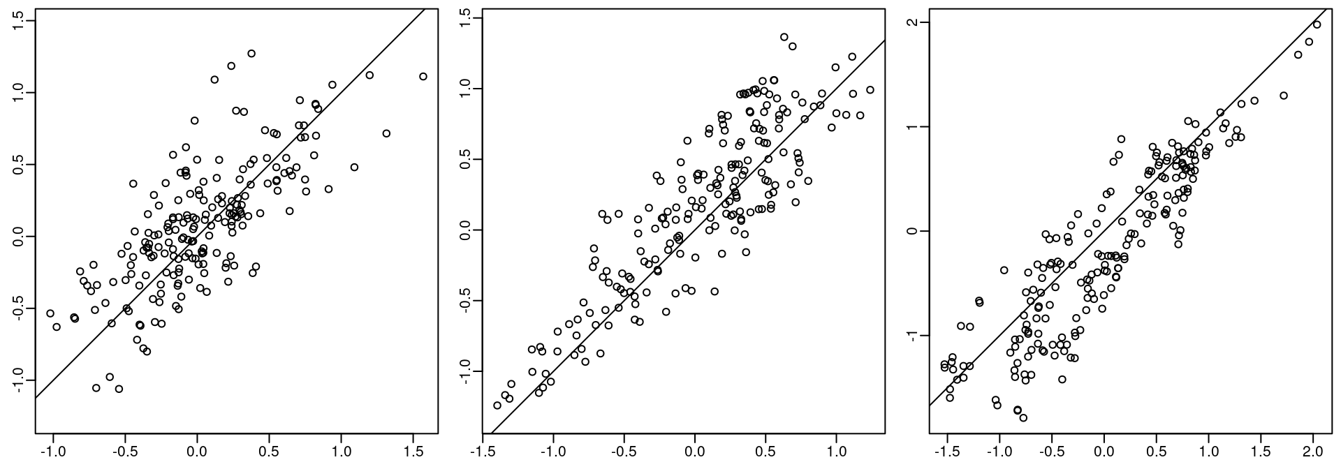
Figure 8.1: True and fitted random field values.
Remember that the crude mesh leads to a crude approximation for the spatial covariance. This is not recommended when fitting a model in practice. However, this setting can be considered to obtain initial results, and for illustrative code examples. In this particular case, it seems that the method provided reasonable estimates of the model parameters.
8.2 Dynamic regression example
There is large literature about dynamic models, which includes some books, such as West and Harrison (1997) and Petris, Petroni, and Campagnoli (2009). These models basically define a hierarchical framework for a class of time series models. A particular case is the dynamic regression model, where the regression coefficients are modeled as time series. That is the case when the regression coefficients vary smoothly over time.
8.2.1 Dynamic space-time regression
The specific class of models for spatially structured time series was proposed in Gelfand et al. (2003), where the regression coefficients vary smoothly over time and space. For the areal data case, the use of proper Gaussian Markov random fields (PGMRF) over space has been proposed in Vivar and Ferreira (2009). There exists a particular class of such models called ``spatially varying coefficient models’’, in which the regression coefficients vary over space. See, for example, Assunção, Gamerman, and Assunção (1999), Assunção, Potter, and Cavenaghi (2002) and Gamerman, Moreira, and Rue (2003).
In Gelfand et al. (2003), the Gibbs sampler was used for inference and it was claimed that a better algorithm is needed due to strong autocorrelations. In Vivar and Ferreira (2009), the use of forward information filtering and backward sampling (FIFBS) recursions were proposed. Both MCMC algorithms are computationally expensive.
The FIFBS algorithm can be avoided as a relation between the Kalman-filter and the Cholesky factorization is proposed in Knorr-Held and Rue (2002). The Cholesky factorization is more general and has a better performance when using sparse matrix methods (p. 149, Rue and Held 2005). Additionally, the restriction that the prior for the latent field has to be proper can be avoided.
When the likelihood is Gaussian, there is no approximation needed in the
inference process since the distribution of the latent field given the data and
the hyperparameters is Gaussian. So, the main task is to perform inference for
the hyperparameters in the model. For this, the mode and curvature around can
be found without any sampling method. For the class of models in Vivar and Ferreira (2009)
it is natural to use INLA, as shown in Ruiz-Cárdenas, Krainski, and Rue (2012), and for the models
in Gelfand et al. (2003), the SPDE approach can be used when considering the Matérn
covariance for the spatial part.
In this example, it will be shown how to fit the space-time dynamic regression model as discussed in Gelfand et al. (2003), considering the Matérn spatial covariance and the AR(1) model for time, which corresponds to the exponential correlation function. This particular covariance choice corresponds to the model in Cameletti et al. (2013), where only the intercept is dynamic. Here, the considered case is that of a dynamic intercept and a dynamic regression coefficient for a harmonic over time.
8.2.2 Simulation from the model
In order to simulate some data to fit the model, the spatial locations are sampled first, as follows:
n <- 150
set.seed(1)
coo <- matrix(runif(2 * n), n)
To sample from a random field at a set of locations, the book.rMatern()
function defined in the Section 2.1.4 will be used to simulate
independent random field realizations for each time.
\(k\) (number of time points) samples will be drawn from the random field. Then, they are temporally correlated considering the time autoregression:
kappa <- c(10, 12)
sigma2 <- c(1 / 2, 1 / 4)
k <- 15
rho <- c(0.7, 0.5)

set.seed(2)
beta0 <- book.rMatern(k, coo, range = sqrt(8) / kappa[1],
  sigma = sqrt(sigma2[1]))

set.seed(3)
beta1 <- book.rMatern(k, coo, range = sqrt(8) / kappa[2],
  sigma = sqrt(sigma2[2]))
beta0[, 1] <- beta0[, 1] / (1 - rho[1]^2)
beta1[, 1] <- beta1[, 1] / (1 - rho[2]^2)

for (j in 2:k) {
  beta0[, j] <- beta0[, j - 1] * rho[1] + beta0[, j] *
    (1 - rho[1]^2)
  beta1[, j] <- beta1[, j - 1] * rho[2] + beta1[, j] *
    (1 - rho[2]^2)
}
Here, the \((1-\rho_j^2)\) term appears because it is in parametrization of the
AR(\(1\)) model in INLA.
To get the response, the harmonic is defined as a function over time, and then the mean and the error terms are added up:
set.seed(4)
# Simulate the covariate values
hh <- runif(n * k)
mu.beta <- c(-5, 1)
taue <- 20

set.seed(5)
# Error in the observation
error <- rnorm(n * k, 0, sqrt(1 / taue))
# Dynamic regression part
y <- (mu.beta[1] + beta0) + (mu.beta[2] + beta1) * hh +
  error
8.2.3 Fitting the model
There are two space-time terms in the model, each one with three hyperparameters: precision, spatial scale and temporal scale (or temporal correlation). So, considering the likelihood precision, there are \(7\) hyperparameters in total. To perform fast inference, a crude mesh with a small number of vertices is chosen:
mesh <- inla.mesh.2d(coo, max.edge = c(0.15, 0.3),
  offset = c(0.05, 0.3), cutoff = 0.07)
This mesh has 195 points.
As in previous examples, the SPDE model will consider the PC-priors derived in Fuglstad et al. (2018) for the model parameters as the practical range, \(\sqrt{8\nu}/\kappa\), and the marginal standard deviation:
spde <- inla.spde2.pcmatern(mesh = mesh,
  prior.range = c(0.05, 0.01), # P(practic.range < 0.05) = 0.01
  prior.sigma = c(1, 0.01)) # P(sigma > 1) = 0.01
A different index is needed for each call to the f()
function, even if they are the same, so:
i0 <- inla.spde.make.index('i0', spde$n.spde, n.group = k)
i1 <- inla.spde.make.index('i1', spde$n.spde, n.group = k)
In the SPDE approach, the space-time model is defined at a set of mesh nodes. As a continuous time is being considered, it is also defined on a set of time knots. So, it is necessary to deal with the projection from the model domain (nodes, knots) to the space-time data locations. For the intercept, it is the same way as in previous examples. For the regression coefficients, all that is required is to multiply the projector matrix by the covariate vector column, i. e., each column of the projector matrix is multiplied by the covariate vector. This can be seen from the following structure of the linear predictor \(\boldeta\):
\[ \begin{array}{rcl} \boldeta & = & \mu_{\beta_0} + \mu_{\beta_2}\mb{h} + \mb{A} \mb{\beta}_0 + (\mb{A} \mb{\beta}_1) \mb{h} \nonumber \\ & = & \mu_{\beta_0} + \mu_{\beta_1}\mb{h} + \mb{A} \mb{\beta}_0 + (\mb{A} \oplus (\mb{h}\mb{1}^{\top}))\mb{\beta}_1 \end{array} \tag{8.1} \]
Here, \(\mb{A} \oplus (\mb{h} \mb{1}^{\top})\) is the row-wise Kronecker product
between \(\mb{A}\) and vector \(\mb{h}\) (with length equal the number of rows in
\(\mb{A}\)) expressed as the Kronecker sum of \(\mb{A}\) and \(\mb{h}\mb{1}^{\top}\).
This operation can be performed using the inla.row.kron() function and is
done internally in the function inla.spde.make.A() when supplying a vector in
the weights argument.
The space-time projector matrix \(\mb{A}\) is defined as follows:
A0 <- inla.spde.make.A(mesh,
  cbind(rep(coo[, 1], k), rep(coo[, 2], k)),
  group = rep(1:k, each = n))
A1 <- inla.spde.make.A(mesh,
  cbind(rep(coo[, 1], k), rep(coo[, 2], k)),
  group = rep(1:k, each = n), weights = hh)
The data stack is as follows:
stk.y <- inla.stack(
  data = list(y = as.vector(y)),
  A = list(A0, A1, 1),
  effects = list(i0, i1, data.frame(mu1 = 1, h = hh)),
  tag = 'y')
Here, i0 is similar to i1 and variables mu1 and h in the second element
of the effects data.frame are for \(\mu_{\beta_0}\), \(\mu_{\beta_1}\) and
\(\mu_{\beta_2}\).
The formula considered in this model takes the following effects into account:
form <- y ~ 0 + mu1 + h + # to fit mu_beta
  f(i0, model = spde, group = i0.group,
    control.group = list(model = 'ar1')) +
  f(i1, model = spde, group = i1.group,
    control.group = list(model = 'ar1'))
As the model considers a Gaussian likelihood, there is no approximation in the fitting process. The first step of the INLA algorithm is the optimization to find the mode of the \(7\) hyperparameters in the model. By choosing good starting values, fewer iterations will be needed in this optimization process. Below, starting values are defined for the hyperparameters in the internal scale considering the values used to simulate the data:
theta.ini <- c(
  log(taue), # likelihood log precision
  log(sqrt(8) / kappa[1]), # log range 1
  log(sqrt(sigma2[1])), # log stdev 1
  log((1 + rho[1])/(1 - rho[1])), # log trans. rho 1
  log(sqrt(8) / kappa[2]), # log range 1
  log(sqrt(sigma2[2])), # log stdev 1
  log((1 + rho[2]) / (1 - rho[2])))# log trans. rho 2

theta.ini
## [1]  2.9957 -1.2629 -0.3466  1.7346 -1.4452 -0.6931  1.0986
The integration step when using the CCD strategy will integrate over 79
hyperparameter configurations, as we have \(7\) hyperparameters. For complex
models, model fitting may take a few minutes. A bigger tolerance value in
inla.control can be set to reduce the number of posterior evaluations, which
will also reduce computational time. However, in the following inla() call
we avoid it by using an Empirical Bayes strategy.
Finally, model fitting considering the initial values defined above will be done as follows:
res <- inla(form, family = 'gaussian',
  data = inla.stack.data(stk.y),
  control.predictor = list(A = inla.stack.A(stk.y)),
  control.inla = list(int.strategy = 'eb'),# no integr. wrt theta
  control.mode = list(theta = theta.ini, # initial theta value
    restart = TRUE))
The time required to fit this model has been:
res$cpu
##      Pre  Running     Post    Total
##   1.0318 355.7276   0.3365 357.0960
Summary of the posterior marginals of \(\mu_{\beta_1}\), \(\mu_{\beta_2}\) and the likelihood precision (i.e., \(1/\sigma^2_e\)) are available in Table 8.2.
| Parameter | True | Mean | St. Dev. | 2.5% quant. | 97.5% quant. |
|---|---|---|---|---|---|
| \(\mu_{\beta_1}\) | -5 | -4.7779 | 0.2004 | -5.1714 | -4.385 |
| \(\mu_{\beta_2}\) | 1 | 0.9307 | 0.0615 | 0.8101 | 1.051 |
| \(1/\sigma^2_e\) | 20 | 10.8897 | 0.4997 | 9.9275 | 11.895 |
The posterior marginal distributions for the range, standard deviation and autocorrelation parameter for each spatio-temporal process are in Figure 8.2.
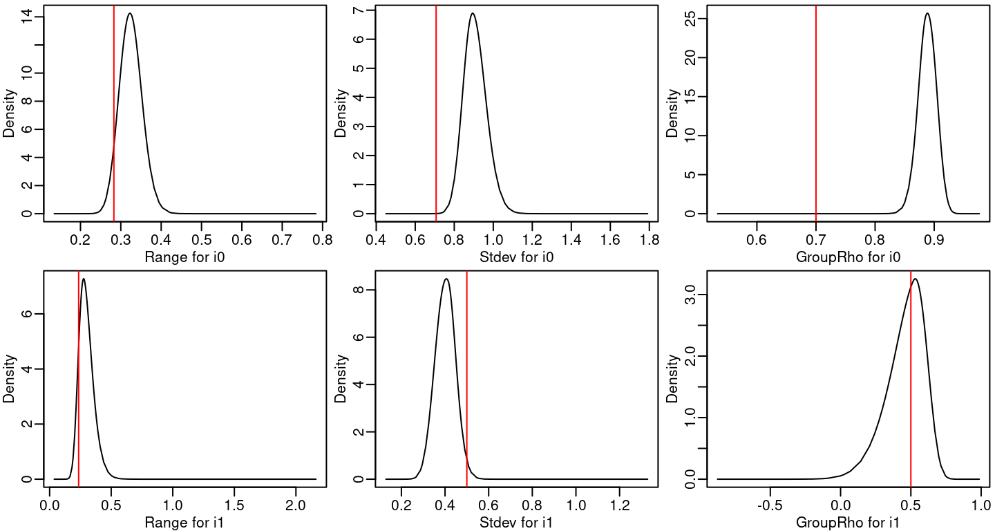
Figure 8.2: Posterior marginal distributions for the hyperparameters of the space-time fields. Red lines represent the true values of the parameters.
In order to look deeper into the posterior means of the dynamic coefficients, the correlation between the mean of the simulated values and the corresponding posterior means have been computed:
## Using A0 to account only for the coeff.
c(beta0 = cor(as.vector(beta0),
    drop(A0 %*% res$summary.ran$i0$mean)),
  beta1 = cor(as.vector(beta1),
    drop(A0 %*% res$summary.ran$i1$mean)))
##  beta0  beta1
## 0.9434 0.6083
8.3 Space-time point process: Burkitt example
In this section a model for space-time point processes is developed and applied to a real dataset.
8.3.1 The dataset
The model developed in this section will be applied in the analysis of the
burkitt dataset from the splancs package (Rowlingson and Diggle 1993). This dataset
records cases of Burkitt’s lymphoma in the Western Nile district of Uganda
during the period 1960-1975 (see, Bailey and Gatrell 1995, Chapter 3).
This dataset contains the five columns described in Table 8.3.
| Variable | Description |
|---|---|
x |
Easting |
y |
Northing |
t |
Day, starting at 1/1/1960 of onset |
age |
age of child patient |
dates |
Day, as string yy-mm-dd |
This dataset can be loaded as follows:
data('burkitt', package = 'splancs')The spatial coordinates and time values can be summarized as follows:
t(sapply(burkitt[, 1:3], summary))
##   Min. 1st Qu. Median   Mean 3rd Qu. Max.
## x  255   269.0  282.5  286.3   300.2  335
## y  247   326.8  344.5  338.8   362.0  399
## t  413  2411.8 3704.5 3529.9  4700.2 5775
A set of knots over time needs to be defined in order to fit a SPDE spatio-temporal model. It is then used to build a temporal mesh, as follows:
k <- 6
tknots <- seq(min(burkitt$t), max(burkitt$t), length = k)
mesh.t <- inla.mesh.1d(tknots)
Figure 8.3 shows the temporal mesh as well as the times at which the events occurred.
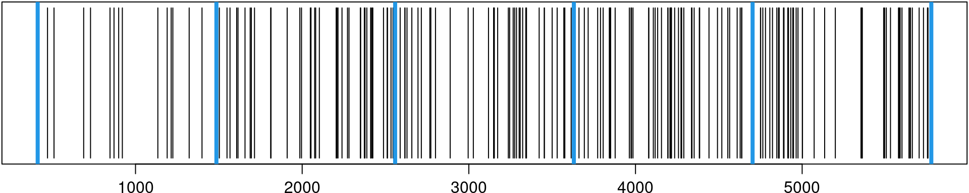
Figure 8.3: Time when each event occurred (black) and knots used for inference (blue).
The spatial mesh can be created using the polygon of the region as a boundary.
The domain polygon can be converted into a
SpatialPolygons class with:
domainSP <- SpatialPolygons(list(Polygons(list(Polygon(burbdy)),
  '0')))
This boundary is then used to compute the mesh:
mesh.s <- inla.mesh.2d(burpts,
  boundary = inla.sp2segment(domainSP),
  max.edge = c(10, 25), cutoff = 5) # a crude mesh
Again, the SPDE model is defined to use the PC-priors derived in Fuglstad et al. (2018) for the range and the marginal standard deviation. These are defined now:
spde <- inla.spde2.pcmatern(mesh = mesh.s,
  prior.range = c(5, 0.01), # P(practic.range < 5) = 0.01
  prior.sigma = c(1, 0.01)) # P(sigma > 1) = 0.01
m <- spde$n.spde
The spatio temporal projection matrix is made considering both spatial and temporal locations and both spatial and temporal meshes, as follows:
Ast <- inla.spde.make.A(mesh = mesh.s, loc = burpts,
  n.group = length(mesh.t$n), group = burkitt$t,
  group.mesh = mesh.t)
The dimension of the resulting projector matrix is:
dim(Ast)
## [1]  188 2424
Internally, the inla.spde.make.A() function makes a row Kronecker product
(see manual page of function inla.row.kron()) between the spatial projector
matrix and the group (temporal dimension, in our case) projector one. This
matrix has number of columns equal to the number of nodes in the mesh times
the number of groups.
The index set is made considering the group feature:
idx <- inla.spde.make.index('s', spde$n.spde, n.group = mesh.t$n)The data stack can be made considering the ideas for the purely spatial model. So, it is necessary to consider the expected number of cases at the integration points and the data locations. For the integration points, it is the space-time volume computed for each mesh node and time knot, considering the spatial area of the dual mesh polygons, as in Chapter 4, times the length of the time window at each time point. For the data locations, it is zero as for a point the expectation is zero, as in the likelihood approximation proposed by Simpson et al. (2016).
The dual mesh is extracted considering function book.mesh.dual(), available
in file spde-book-functions.R, as follows:
dmesh <- book.mesh.dual(mesh.s)Then, the intersection with each polygon from the dual mesh is computed using
functions gIntersection(), from the rgeos package, as:
library(rgeos)
w <- sapply(1:length(dmesh), function(i) {
  if (gIntersects(dmesh[i,], domainSP))
    return(gArea(gIntersection(dmesh[i,], domainSP)))
  else return(0)
})
The sum of all the weights is equal to \(1.1035\times 10^{4}\). This is the same as the domain area:
gArea(domainSP)
## [1] 11035
The spatio-temporal volume is the product of these values and the time window length of each time knot. It is computed here:
st.vol <- rep(w, k) * rep(diag(inla.mesh.fem(mesh.t)$c0), m)The data stack is built using the following lines of R code:
y <- rep(0:1, c(k * m, n))
expected <- c(st.vol, rep(0, n))
stk <- inla.stack(
  data = list(y = y, expect = expected),
  A = list(rbind(Diagonal(n = k * m), Ast), 1),
  effects = list(idx, list(a0 = rep(1, k * m + n))))
Finally, model fitting will be done using the cruder Gaussian approximation:
pcrho <- list(prior = 'pc.cor1', param = c(0.7, 0.7))
form <- y ~ 0 + a0 + f(s, model = spde, group = s.group,
  control.group = list(model = 'ar1',
    hyper = list(rho = pcrho)))

burk.res <- inla(form, family = 'poisson',
  data = inla.stack.data(stk), E = expect,
  control.predictor = list(A = inla.stack.A(stk)),
  control.inla = list(strategy = 'adaptive'))
The exponential of the intercept plus the random effect at each space-time
integration point is the relative risk at each of these points. This relative
risk times the space-time volume will give the expected number of points
(E(n)) at each one of these space-time locations. Summing over them will
give a value that approaches the number of observations:
eta.at.integration.points <- burk.res$summary.fix[1,1] +
   burk.res$summary.ran$s$mean
c(n = n, 'E(n)' = sum(st.vol * exp(eta.at.integration.points)))
##     n  E(n)
## 188.0 144.8
The posterior marginal distributions for the intercept and the other parameters in the model have been plotted in Figure 8.4.
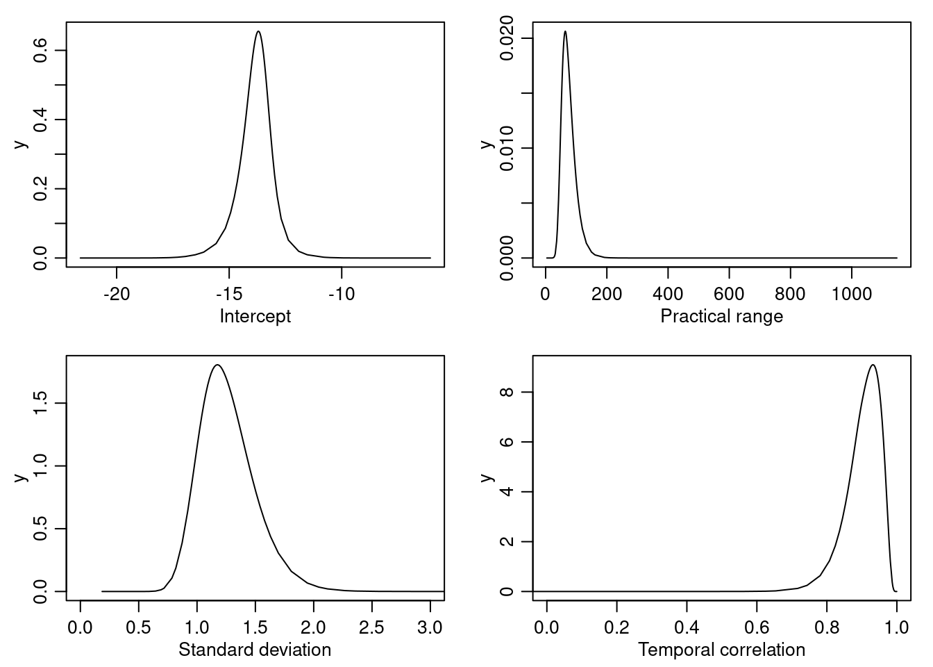
Figure 8.4: Intercept and random field parameters posterior marginal distributions.
The projection over a grid for each time knot can be computed as:
r0 <- diff(range(burbdy[, 1])) / diff(range(burbdy[, 2]))
prj <- inla.mesh.projector(mesh.s, xlim = range(burbdy[, 1]),
  ylim = range(burbdy[, 2]), dims = c(100, 100 / r0))
ov <- over(SpatialPoints(prj$lattice$loc), domainSP)
m.prj <- lapply(1:k, function(j) {
  r <- inla.mesh.project(prj,
    burk.res$summary.ran$s$mean[1:m + (j - 1) * m])
  r[is.na(ov)] <- NA
  return(r)
})
The fitted latent field at each time knot has been displayed in Figure 8.5. A similar plot could be produced for the standard deviation.
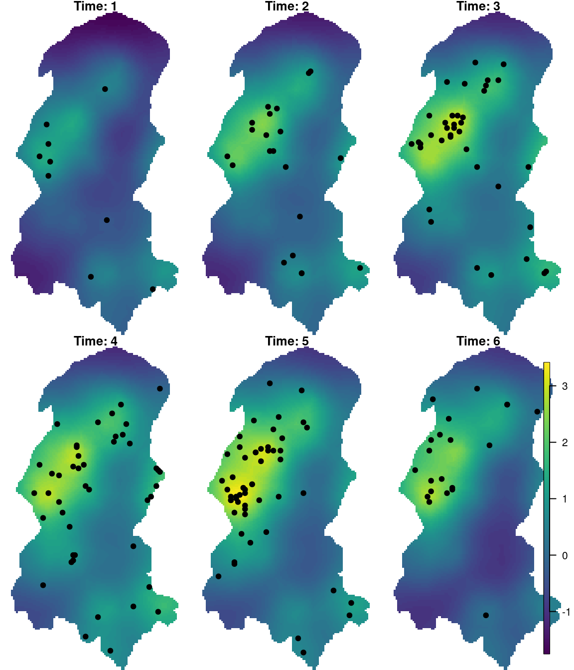
Figure 8.5: Fitted latent field at each time knot overlayed by the points closer in time.
8.4 Large point process dataset
In this section an approach to fit a spatio-temporal log-Gaussian Cox point process model for a large dataset is shown using a simulated dataset.
8.4.1 Simulated dataset
The dataset will be simulated by drawing samples from a separable space-time intensity function. We assume that the logarithm of the intensity function is a Gaussian process. This space-time point process can be sampled in two steps. First, a sample from a separable spacetime Gaussian process is drawn. Second, the point process is sampled conditional to this realization.
The separable space-time covariance assumed considers a Matérn covariance for space and the Exponential for time. In this case the temporal correlation at lag \(\delta t\) is \(\textrm{e}^{-\theta \delta t}\). Considering this continuous process sampled at equally spaced intervals \(t_1, t_2, ...\), with \(t_2-t_1=\delta t\), then the correlation can be expressed as \(\rho=\textrm{e}^{-\theta \delta t}\). If \(\delta t=1\) we have \(\rho=\textrm{e}^{-\theta}\). This establishes a link with the first order autoregression that we will consider in the fitting process, where \(\rho\) is the lag one correlation parameter.
The sample is drawn using the lgcp package (Taylor et al. 2013).
We have to specify the parameters for the Gaussian process.
These are the marginal standard deviation \(\sigma\),
the spatial correlation parameter \(\phi\) (which gives us
\(\sqrt{\phi}\) as the spatial range in our parametrization)
and the temporal correlation parameter \(\theta=-\log(\rho)\).
These parameters are passed to the lgcpSim() function considering the
lgcppars() function.
There are two additional parameters for the lgcpSim() function which are
related to the mean of the Gaussian latent process, the intercept \(\mu\) and
\(\beta\) that is used in case of covariate. We can increase \(\mu\) in order to
increase the intensity function and then increase the number of points in the
sample. The expected number of points in the sample depends on the mean of the
intensity function which is modeled by the mean of the latent field, the
variance of the latent field, the size of the spatial domain and the length of
the time window as \(\textrm{E}(N) = \exp(\mu + \sigma^2/2) * V\), where \(V\) is
the area of the spatial domain times the time length.
First, the spatial domain is defined as follows:
x0 <- seq(0, 4 * pi, length = 15)
domain <- data.frame(x = c(x0, rev(x0), 0))
domain$y <- c(sin(x0 / 2) - 2, sin(rev(x0 / 2)) + 2, sin(0) - 2)
Then, it is converted into an object of the SpatialPolygons class:
domainSP <- SpatialPolygons(list(Polygons(list(Polygon(domain)),
  '0')))
The area can be computed as:
library(rgeos)
s.area <- gArea(domainSP)
We can now define the model parameters:
ndays <- 12

sigma <- 1
phi <- 1
range <- sqrt(8) * phi
rho <- 0.7
theta <- -log(rho)
mu <- 2

(E.N <- exp(mu + sigma^2/2) * s.area * ndays )
## [1] 7348
Then we use the lgcpSim() function to sample the points:
if(require("lgcp", quietly = TRUE)) {
    mpars <- lgcppars(sigma, phi, theta, mu - sigma^2/2)
    set.seed(1)
    xyt <- lgcpSim(
      owin = spatstat.geom:::owin(poly = domain), tlim = c(0, ndays),
      model.parameters = mpars, cellwidth = 0.1,
      spatial.covmodel = 'matern', covpars = c(nu = 1))
  #save("xyt", file="data/xyt.RData")
} else {
  load("data/xyt.RData")
}

n <- xyt$n
In the previous code we have used the require() function to check whether the
lgcp package can be loaded. The lgcp package depends on the rpanel
package (Bowman et al. 2010) which in turn depends on the TCL/TK widget library
BWidget. This is a system dependence, which cannot be installed from R, and
may not be available on all systems by default. In case the BWidget library
is not installed locally, the lgcp package will fail to install and the code
above cannot be run, but the simulated data can be downloaded from the book
website in order to run the examples below.
In order to fit the model, a discretization over space and over time needs to be defined. For the temporal domain, a temporal mesh based on a number of time knots will be used:
w0 <- 2
tmesh <- inla.mesh.1d(seq(0, ndays, by = w0))
tmesh$loc
## [1]  0  2  4  6  8 10 12
(k <- length(tmesh$loc))
## [1] 7
In order to consider fast computations, we lower the mesh resolution. However, it has to be tuned with the range of the spatial process. One should think about the problem of having a too coarse mesh that may not represent the Matérn field. One way to consider this is to try with a coarse mesh and look at the estimated range and then improve from there if necessary. It is better to avoid having the spatial range smaller than the mesh edge length.
The spatial mesh is defined using the domain polygon:
smesh <- inla.mesh.2d(boundary = inla.sp2segment(domainSP),
  max.edge = 0.75, cutoff = 0.3)
Figure 8.6 shows a plot of a sample of the data over time and the time knots, as well as a plot of the data over space and the spatial mesh.
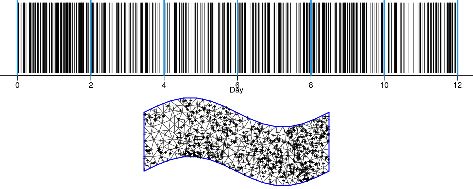
Figure 8.6: Time for a sample of the events (black), time knots (blue) in the upper plot. Spatial locations of another sample on the spatial domain (bottom plot).
8.4.2 Space-time aggregation
For large datasets it can be computationally demanding to fit the model. The problem is that the dimension of the model will be \(n + m * k\), where \(n\) is the number of data points, \(m\) is the number of nodes in the mesh and \(k\) is the number of time knots. In this section the approach chosen to deal with the model is to aggregate the data in a way that the problem is reduced to one of dimension \(2*m*k\). So, this approach really makes sense when \(n\gg m*k\).
Data will be aggregated according to the integration points to make the fitting process easier. Dual mesh polygons will also be considered, as shown in Chapter 4.
So, the first step is to find the Voronoi polygons for the mesh nodes:
library(deldir)
dd <- deldir(smesh$loc[, 1], smesh$loc[, 2])
tiles <- tile.list(dd)
Then, these are converted into a SpatialPolygons object, as follows:
polys <- SpatialPolygons(lapply(1:length(tiles), function(i) {
  p <- cbind(tiles[[i]]$x, tiles[[i]]$y)
  n <- nrow(p)
  Polygons(list(Polygon(p[c(1:n, 1), ])), i)
}))
The next step is to find to which polygon each data point belongs:
area <- factor(over(SpatialPoints(cbind(xyt$x, xyt$y)), polys),
  levels = 1:length(polys))
Similarly, it is necessary to find to which part of the time mesh each data point belongs:
t.breaks <- sort(c(tmesh$loc[c(1, k)],
  tmesh$loc[2:k - 1] / 2 + tmesh$loc[2:k] / 2))
time <- factor(findInterval(xyt$t, t.breaks),
  levels = 1:(length(t.breaks) - 1))
The distribution of data points on the time knots is summarized here:
table(time)
## time
##    1    2    3    4    5    6    7
##  657 1334  845  782  832 1022  610
Then, both identification index sets are used to aggregate the data:
agg.dat <- as.data.frame(table(area, time))
for(j in 1:2) # set time and area as integer
    agg.dat[[j]] <- as.integer(as.character(agg.dat[[j]]))
The resulting data.frame contains the area, time span and frequency of the
aggregated data:
str(agg.dat)
## 'data.frame':    1715 obs. of  3 variables:
##  $ area: int  1 2 3 4 5 6 7 8 9 10 ...
##  $ time: int  1 1 1 1 1 1 1 1 1 1 ...
##  $ Freq: int  2 0 0 1 1 0 0 2 4 0 ...
The expected number of cases needs to be defined (at least) proportional to the area of the polygons times the width length of the time knots. Computing the intersection area of each polygon with the domain (show the sum) is done as follows:
w.areas <- sapply(1:length(tiles), function(i) {
  p <- cbind(tiles[[i]]$x, tiles[[i]]$y)
  n <- nrow(p)
  pl <- SpatialPolygons(
    list(Polygons(list(Polygon(p[c(1:n, 1),])), i)))
  if (gIntersects(pl, domainSP))
    return(gArea(gIntersection(pl, domainSP)))
  else return(0)
})
A summary of the areas of the polygons is:
summary(w.areas)
##    Min. 1st Qu.  Median    Mean 3rd Qu.    Max.
##   0.039   0.137   0.215   0.205   0.256   0.350
The total sum of the weights is \(50.2655\) and the area of the spatial domain is:
s.area
## [1] 50.27
The time length (domain) is 12 and the width of each knot is
w.t <- diag(inla.mesh.fem(tmesh)$c0)
w.t
## [1] 1 2 2 2 2 2 1
Here, the knots at the boundaries of the time period have a lower width than the internal ones.
Since the intensity function is the number of cases per volume unit, with \(n\) cases the intensity varies about the average number of cases (intensity) by unit volume. This quantity is related to the intercept in the model. Actually, the log of it is an estimative of the intercept in the model without the space-time effect. See below:
i0 <- n / (gArea(domainSP) * diff(range(tmesh$loc)))
c(i0, log(i0))
## [1] 10.083  2.311
The space-time volume (area unit per time unit) at each polygon and time knot is:
e0 <- w.areas[agg.dat$area] * (w.t[agg.dat$time])
summary(e0)
##    Min. 1st Qu.  Median    Mean 3rd Qu.    Max.
##   0.039   0.226   0.347   0.352   0.483   0.700
8.4.3 Model fitting
The projector matrix, SPDE model object and the space-time index set definition are computed as follows:
A.st <- inla.spde.make.A(smesh, smesh$loc[agg.dat$area, ],
  group = agg.dat$time, mesh.group = tmesh)
spde <- inla.spde2.pcmatern(
  smesh, prior.sigma = c(1,0.01), prior.range = c(0.05,0.01))
idx <- inla.spde.make.index('s', spde$n.spde, n.group = k)
The data stack is defined as:
stk <- inla.stack(
  data = list(y = agg.dat$Freq, exposure = e0),
  A = list(A.st, 1),
  effects = list(idx, list(b0 = rep(1, nrow(agg.dat)))))
The formula to fit the model considers the intercept, spatial effect and temporal effect:
# PC prior on correlation
pcrho <- list(rho = list(prior = 'pc.cor1', param = c(0.7, 0.7)))
# Model formula
formula <- y ~ 0 + b0 +
  f(s, model = spde, group = s.group,
    control.group = list(model = 'ar1', hyper = pcrho))
Finally, model fitting is carried out:
res <- inla(formula, family = 'poisson',
  data = inla.stack.data(stk), E = exposure,
  control.predictor = list(A = inla.stack.A(stk)),
  control.inla = list(strategy ='adaptive'))
The value of \(\mu\) and the intercept summary can be obtained as follows:
cbind(True = mu, res$summary.fixed[, 1:6])
##    True  mean     sd 0.025quant 0.5quant 0.975quant  mode
## b0    2 2.043 0.1762      1.695    2.042      2.392 2.041
The expected number of cases at each integration point can be used to compute
the total expected number of cases (Est. N below), as:
eta.i <- res$summary.fix[1, 1] + res$summary.ran$s$mean
c('E(N)' = E.N, 'Obs. N' = xyt$n,
  'Est. N' = sum(rep(w.areas, k) *
     rep(w.t, each = smesh$n) * exp(eta.i)))
##   E(N) Obs. N Est. N
##   7348   6082   5726
A summary for the hyperparameters can be obtained with this R code:
cbind(True = c(range, sigma, rho),
  res$summary.hyperpar[, c(1, 2, 3, 5)])
##                 True   mean      sd 0.025quant 0.975quant
## Range for s    2.828 2.4290 0.19601     2.0767     2.8470
## Stdev for s    1.000 0.6791 0.03894     0.6073     0.7605
## GroupRho for s 0.700 0.5286 0.04526     0.4379     0.6156
The spatial surface at each time knot can be computed as well:
r0 <- diff(range(domain[, 1])) / diff(range(domain[, 2]))
prj <- inla.mesh.projector(smesh, xlim = bbox(domainSP)[1, ],
  ylim = bbox(domainSP)[2, ], dims = c(r0 * 200, 200))
g.no.in <- is.na(over(SpatialPoints(prj$lattice$loc), domainSP))
t.mean <- lapply(1:k, function(j) {
  z.j <- res$summary.ran$s$mean[idx$s.group == j]
  z <- inla.mesh.project(prj, z.j)
  z[g.no.in] <- NA
  return(z)
})
Figure 8.7 shows the predicted surfaces at each time knot.
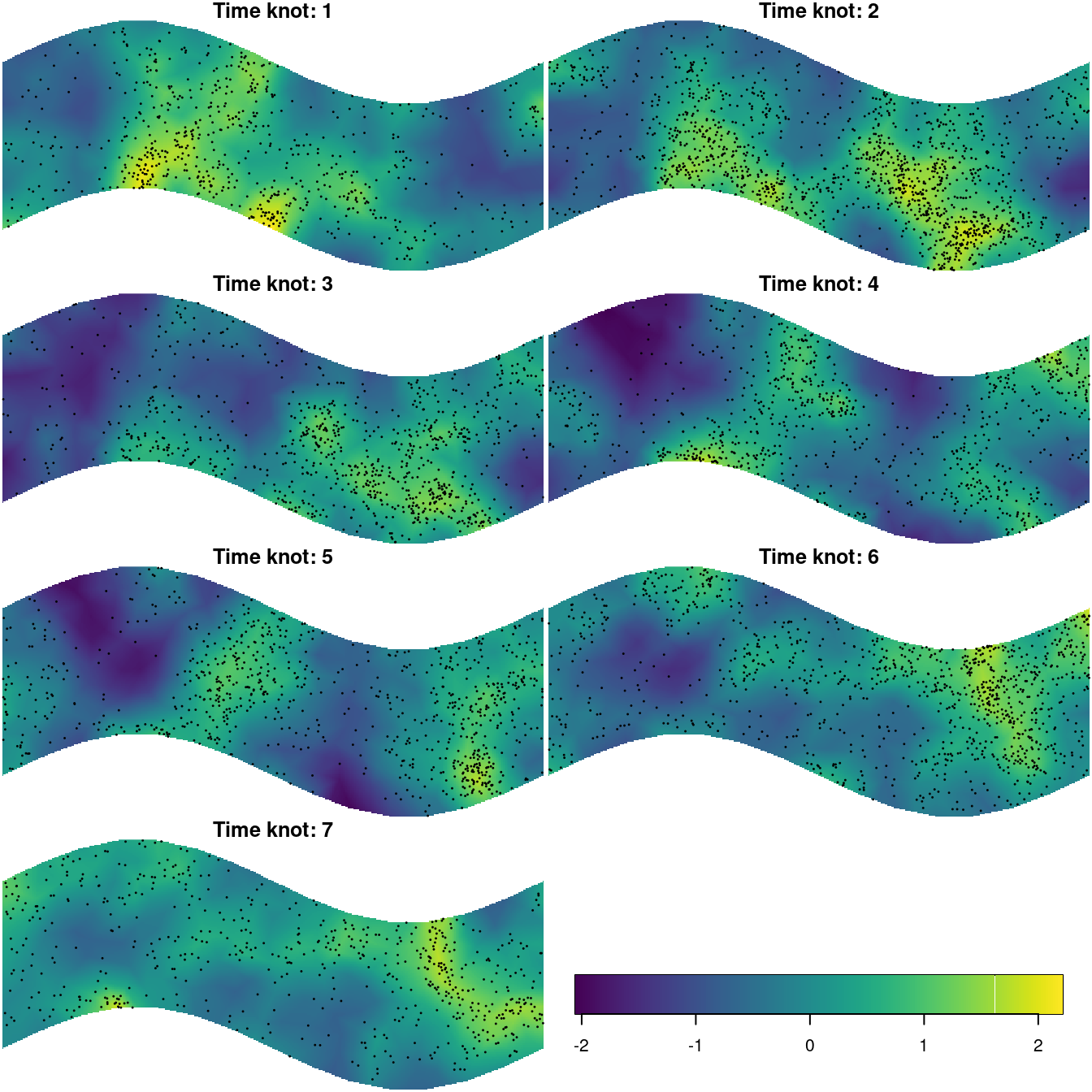
Figure 8.7: Spatial surface fitted at each time knot overlayed by the point pattern formed by the points nearest to each time knot.
8.5 Accumulated rainfall: Hurdle Gamma model
For some applications it is possible to have the outcome be zero or a positive number. Common examples are fish biomass and accumulated rainfall. In this case one can build a model that accommodates the zero and positive outcome considering a combination of two likelihoods, one to model the occurrence and another to model the amount. One case is when considering the Bernoulli distribution for the occurrence and the Gamma for the amount. The advantage of having this two-part model is that we can model the probability of rain and the rainfall amount separately. It may be the case that some terms in each part can be shared.
8.5.1 The model
We will consider the daily rainfall data considered in Section 2.8. Let
\[\begin{align} z_{i,t} = \begin{cases} 1, & \text{ if it has rained at location } \textbf{s}_i \text{ and time } t \\ \\ 0, & \text{otherwise} \end{cases} \end{align}\]
and the rainfall amount as
\[\begin{align} y_{i,t} = \begin{cases} \text{NA}, &\text{if it did not rain at}\\ & \text{location } \textbf{s}_i \text{ and time } t\\ \text{rainfall amount at location } \textbf{s}_i \text{ and time } t, & \text{otherwise} \end{cases} \end{align}\]
We then define a likelihood for each outcome. We choose to set a Bernoulli distribution for \(z_i\) and a Gamma distribution for \(y_i\):
\[\begin{align} z_{i,t} \sim \text{Binomial}(\pi_{i,t},n_{i,t}=1) \;\;\;\text{and}\;\;\;\; y_{i,t} \sim \text{Gamma}(a_{i,t}, b_{i,t}). \end{align}\]
This setting is equivalent to consider a Hurdle-Gamma model where we have the expected value of the rainfall as \(\pi_{i,t}\mu_{i,t}\) where \(\mu_{i,t}\) is the expected value for the Gamma part. Next, we define the model for \(\pi_{i,t}\) and \(\mu_{i,t}\).
For the occurrence, the model is for the linear predictor as the logit of the probability as usual for the Bernoulli, specified as
\[\begin{equation} \tag{8.2} \text{logit}(\pi_{i,t}) = \alpha^z + \xi_{i,t} \end{equation}\]
with \(\alpha^z\) being the intercept and \(\xi_i\) coming from a space-time random effect, i.e. a GF modeled through the SPDE approach.
The parameterization of the Gamma distribution in R-INLA
considers that E\((y) = \mu = a/b\) and Var\((y) = a/b^2=1/\tau\),
where \(\tau\) is the precision parameter.
The linear predictor is defined on \(\log(\mu)\) and we have
\[\begin{equation} \tag{8.3} \log(\mu_{i,t}) = \alpha^y + \beta \xi_{i,t} + u_{i,t} \end{equation}\]
where \(\alpha^y\) is the intercept and \(\beta\) the scaling parameter for \(\xi_{i,t}\), which is the space-time effect considered for the occurrence probability, which is being shared in the model for the rainfall amount. The linear predictor affects both the E\((y)\) and Var\((y)\) because \(a=b\mu\) and then \(a/b^2=\mu/b\).
Notice that \(\xi_{i,t}\) will be computed as \(\xi_{i,t}\mathbf{A}\xi_0\), where \(\xi_0\) is the space-time process at the mesh nodes and time points and \(\mathbf{A}\) is the correspondent space-time projector matrix. This is similar for \(u_{i,t}\).
We will consider the model in Cameletti et al. (2013) for both \(\mathbf{\xi}\) and \(\mathbf{u}\). However, we will consider the PC-prior for each one of the three parameters. Thus for the marginal standard deviation and the spatial range we consider the prior proposed in Fuglstad et al. (2018). We set it such that the standard deviation median is 0.5, \(P(\sigma>0.5=0.5)\).
psigma <- c(0.5, 0.5)For the practical range we consider the size of the Parana state. First we load the data which also load the Parana border, .
data(PRprec)
head(PRborder,2)
##      Longitude Latitude
## [1,]    -54.61   -25.45
## [2,]    -54.60   -25.43
We consider that the coordinates are in longitude and latitude and project them into UTM with units in kilometers as follows:
border.ll <- SpatialPolygons(list(Polygons(list(
  Polygon(PRborder)), '0')),
  proj4string = CRS("+proj=longlat +datum=WGS84"))
border <- spTransform(border.ll,
  CRS("+proj=utm +units=km +zone=22 +south"))
bbox(border)
##    min    max
## x  136  799.9
## y 7045 7509.6
apply(bbox(border), 1, diff)
##     x     y
## 663.9 464.7
We have that the Paraná state is around 663.8711 kilometers width by 464.7481 kilometers height. The PC-prior for the practical range is built considering the probability of the practical range being less than a chosen distance. We chose to set the prior considering the median as 100 kilometers.
prange <- c(100, 0.5)For the temporal correlation parameter, the first order autoregression parameter, we also consider the PC-prior framework, as in Simpson et al. (2016). We choose to have the correlation one as the base model and set the prior considering P(\(\rho>0.5\))=0.7 as follows:
rhoprior <- list(rho = list(prior = 'pc.cor1',
  param = c(0.5, 0.7)))
For the shared parameter \(\beta\) we can set a prior based on some knowledge about the correlation between the rain occurrence and the rainfall amount. We assume a N(0, 1) prior for this parameter as follows
bprior <- list(prior = 'gaussian', param = c(0,1))We also have a likelihood parameter to set prior on and, again, we consider the PC-prior framework. Thus we set the prior on the precision choosing a value for \(\lambda\). We consider it equals one as follows:
pcgprior <- list(prior = 'pc.gamma', param = 1)8.5.2 Rainfall data in Paraná
In this section we consider the rainfall data introduced in Section 2.8. In this data we have the longitude in the first column, the latitude in the second, the altitude in the third and from the fourth column we have the data for each day, as we can see below:
PRprec[1:3, 1:8]
##   Longitude Latitude Altitude d0101 d0102 d0103 d0104 d0105
## 1    -50.87   -22.85      365     0     0     0   0.0     0
## 3    -50.77   -22.96      344     0     1     0   0.0     0
## 4    -50.65   -22.95      904     0     0     0   3.3     0
loc.ll <- SpatialPoints(PRprec[,1:2], border.ll@proj4string)
loc <- spTransform(loc.ll, border@proj4string)
We will consider the first 8 days of data for illustration. The two response variables \(z_i\) and \(y_i\) are defined as follows. First we define the occurrence variable
m <- 8
days.idx <- 3 + 1:m
z <- as.numeric(PRprec[, days.idx] > 0)
table(z)
## z
##    0    1
## 3153 1719
The rainfall is then defined as
y <- ifelse(z == 1, unlist(PRprec[, days.idx]), NA)
table(is.na(y))
##
## FALSE  TRUE
##  1719  3209
8.5.3 Fitting the model
We have to build a mesh in order to define the SPDE model. We consider all the gauges’ locations in the following code:
mesh <- inla.mesh.2d(loc, max.edge = 200, cutoff = 35,
  offset = 150)
And we have the resulting mesh in Figure 8.8.
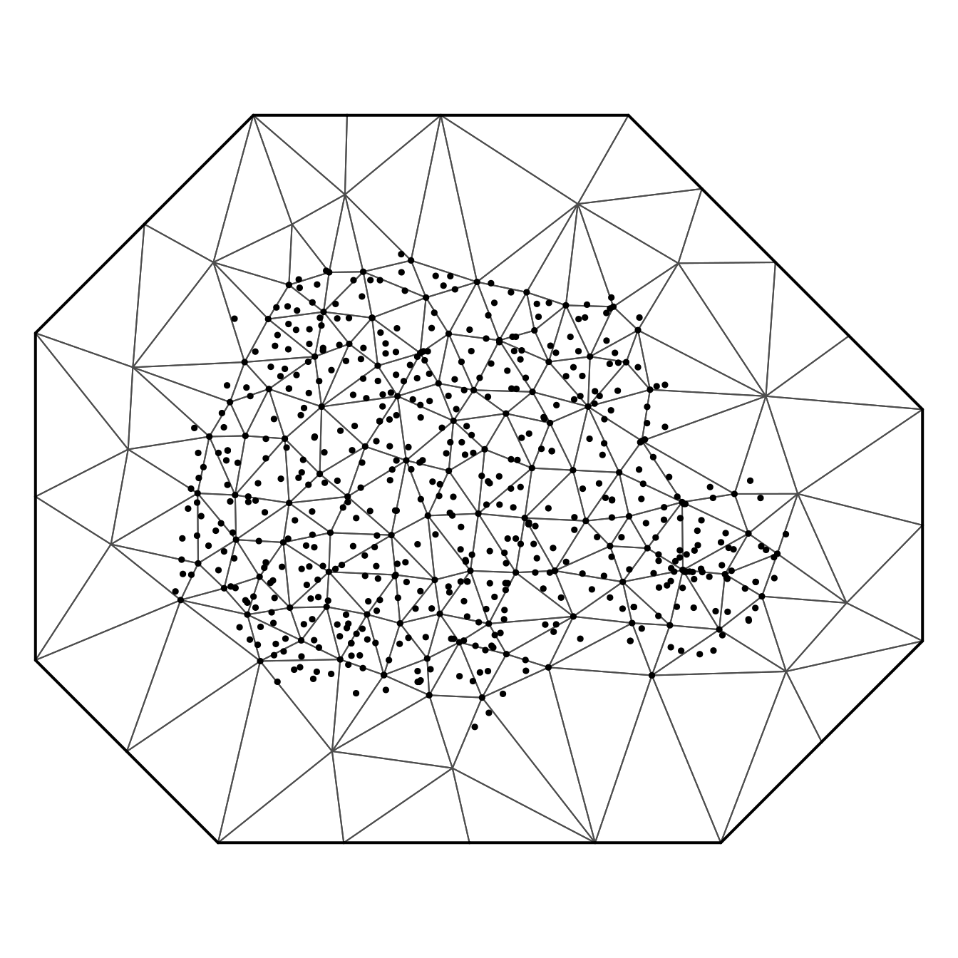
Figure 8.8: Mesh for the Paraná state with 138 nodes. Black points denote the 616 rain gauges.
The SPDE model is defined through
spde <- inla.spde2.pcmatern(
  mesh, prior.range = prange, prior.sigma = psigma)
and the corresponding spacetime predictor matrix is given by
n <- nrow(PRprec)
stcoords <- kronecker(matrix(1, m, 1), coordinates(loc))
A <- inla.spde.make.A(mesh = mesh, loc = stcoords,
  group = rep(1:m, each = n))
dim(A) == (m * c(n, spde$n.spde)) # Check that dimensions match
## [1] TRUE TRUE
We need to define the space-time indices \(\mathbf{\xi}\) in both the linear predictors.
field.z.idx <- inla.spde.make.index(name = 'x',
  n.spde = spde$n.spde, n.group = m)
field.zc.idx <- inla.spde.make.index(name = 'xc',
  n.spde = spde$n.spde, n.group = m)
field.y.idx <- inla.spde.make.index(name = 'u',
  n.spde = spde$n.spde, n.group = m)
The next step is to organize the data into stacks. First, we create a data stack for the occurrence data bearing in mind that we have the amount data. So, we have the occurrence in the first column of a two-column matrix and the amount of rainfall in the second column:
stk.z <- inla.stack(
  data = list(Y = cbind(as.vector(z), NA), link = 1),
  A = list(A, 1),
  effects = list(field.z.idx, z.intercept = rep(1, n * m)),
  tag = 'zobs')

stk.y <- inla.stack(
  data = list(Y = cbind(NA, as.vector(y)), link = 2),
  A = list(A, 1),
  effects = list(c(field.zc.idx, field.y.idx),
  y.intercept = rep(1, n * m)),
  tag = 'yobs')
It is useful to have a stack for prediction at the mesh nodes so it will be easy to map the predicted values later:
stk.zp <- inla.stack(
  data = list(Y = matrix(NA, ncol(A), 2), link = 1),
  effects = list(field.z.idx, z.intercept = rep(1, ncol(A))),
  A = list(1, 1),
  tag = 'zpred')

stk.yp <- inla.stack(
  data = list(Y = matrix(NA, ncol(A), 2), link = 2),
  A = list(1, 1),
  effects = list(c(field.zc.idx, field.y.idx),
    y.intercept = rep(1, ncol(A))),
  tag = 'ypred')
We join all the data stacks:
stk.all <- inla.stack(stk.z, stk.y, stk.zp, stk.yp)We now set some parameters to supply for the inla() function. The prior for
the precision parameter of the Gamma likelihood will go in a list for control
family arguments.
cff <- list(list(), list(hyper = list(prec = pcgprior)))Note that the empty list above, i.e., list(), is required and it could be
used to pass additional arguments to the Binomial likelihood in the model.
For having a fast approximation of the marginals we use the adaptive
approximation strategy (by setting strategy = 'adaptive' below). This
strategy mostly uses the Gaussian approximation to avoid the second Laplace
approximation in the INLA algorithm, but applies the default strategy for fixed
effects and random effects with a length \(\leq\) adaptive.max (see
?control.inla). Additionally we choose to not integrate over the
hyperparameters by choosing the Empirical Bayes estimation as int.strategy = 'eb'. These options will be passed in argument control.inla to function
inla() when fitting the model and are defined now:
cinla <- list(strategy = 'adaptive', int.strategy = 'eb') We also consider not to return the marginal distribution for the latent field. Thus we set
cres <- list(return.marginals.predictor = FALSE,
  return.marginals.random = FALSE)
We can define the model formula for the model specified. We use the spde
object to define the model of the space-time component together with the
definition of the prior for the AR(\(1\)) temporal dynamics. In order to define the
\(\beta\) parameter of the shared space-time component we set fixed = FALSE to
estimate \(\beta\) and insert its prior. In order to achieve fewer iterations
during the optimization over the posterior for the hyperparameters we set
initial values near the optimal ones as we have run this model previously, and
restart the optimization from there. The joint model with the shared
space-time component is then fitted as follows:
cg <- list(model = 'ar1', hyper = rhoprior)
formula.joint <- Y ~ -1 + z.intercept + y.intercept +
  f(x, model = spde, group = x.group, control.group = cg) +
  f(xc, copy = "x", fixed = FALSE, group = xc.group,
    hyper = list(beta = bprior)) +
  f(u, model = spde, group = u.group, control.group = cg)

# Initial values of parameters
ini.jo <- c(-0.047, 5.34, 0.492, 1.607, 4.6, -0.534, 1.6, 0.198)

res.jo <- inla(formula.joint, family = c("binomial", "gamma"),
  data = inla.stack.data(stk.all), control.family = cff,
  control.predictor = list(A = inla.stack.A(stk.all),
    link = link),
  control.compute = list(dic = TRUE, waic = TRUE, cpo = TRUE,
    config = TRUE),
  control.results = cres, control.inla = cinla,
  control.mode = list(theta = ini.jo, restart = TRUE))
The model without the shared space-time component is fitted as follows:
formula.zy <- Y ~ -1 + z.intercept + y.intercept +
  f(x, model = spde, group = x.group, control.group = cg) +
  f(u, model = spde, group = u.group, control.group = cg)

# Initial values of parameters
ini.zy <- c(-0.05, 5.3, 0.5, 1.62, 4.65, -0.51, 1.3)

res.zy <- inla(formula.zy, family = c("binomial", "gamma"),
  data = inla.stack.data(stk.all), control.family = cff,
  control.predictor = list(A =inla.stack.A(stk.all),
    link = link),
  control.compute=list(dic = TRUE, waic = TRUE, cpo = TRUE,
    config = TRUE),
  control.results = cres, control.inla = cinla,
  control.mode = list(theta = ini.zy, restart = TRUE))
Alternatively, the model with only the shared component is fitted as follows:
formula.sh <- Y ~ -1 + z.intercept + y.intercept +
  f(x, model = spde, group = x.group, control.group = cg) +
  f(xc, copy = "x", fixed = FALSE, group = xc.group)

# Initial values of parameters
ini.sh <- c(-0.187, 5.27, 0.47, 1.47, 0.17)

res.sh <- inla(formula.sh, family = c("binomial", "gamma"),
  data = inla.stack.data(stk.all), control.family = cff,
  control.predictor = list(
    A = inla.stack.A(stk.all), link = link),
  control.compute = list(dic = TRUE, waic = TRUE, cpo = TRUE,
    config = TRUE),
  control.results = cres, control.inla = cinla,
  control.mode = list(theta = ini.sh, restart = TRUE))
Sometimes, the CPO is not computed automatically for all the observations.
In this case we can use the inla.cpo() function to manually compute it.
sum(res.jo$cpo$failure, na.rm = TRUE)
sum(res.zy$cpo$failure, na.rm = TRUE)
sum(res.sh$cpo$failure, na.rm = TRUE)

res.jo <- inla.cpo(res.jo, verbose = FALSE)

res.zy <- inla.cpo(res.zy, verbose = FALSE)
res.sh <- inla.cpo(res.sh, verbose = FALSE)
We can now perform a model comparison. This can be done using the marginal likelihood, DIC, WAIC or CPO. Because we have two outcomes, we need to account for this with care. The DIC, WAIC and CPO are computed for each observation. Thus, we can sum it for each outcome as follows:
getfit <- function(r) {
  fam <- r$dic$family
  data.frame(dic = tapply(r$dic$local.dic, fam, sum),
    waic = tapply(r$waic$local.waic, fam, sum),
    cpo = tapply(r$cpo$cpo, fam,
      function(x) - sum(log(x), na.rm = TRUE)))
}
rbind(separate = getfit(res.jo),
  joint = getfit(res.zy),
  oshare = getfit(res.sh))[c(1, 3, 5, 2, 4, 6),]
##              dic  waic  cpo
## separate.1  5094  5082 2542
## joint.1     5097  5084 2543
## oshare.1    5101  5088 2545
## separate.2 11282 11297 5693
## joint.2    11293 11310 5706
## oshare.2   11457 11458 5729
and we can see that the separate model fits slightly better.
8.5.4 Visualizing some results
We extract the useful indices for later use, one for each outcome at the observation locations and one for each outcome at the mesh locations, for all time points:
idx.z <- inla.stack.index(stk.all, 'zobs')$data
idx.y <- inla.stack.index(stk.all, 'yobs')$data
idx.zp <- inla.stack.index(stk.all, 'zpred')$data
idx.yp <- inla.stack.index(stk.all, 'ypred')$data
It may be useful to show maps of the space-time effect at each time, or the probability of rain or the expected value of rainfall. In order to compute it we do need to have the projector from the mesh nodes to a fine grid:
wh <- apply(bbox(border), 1, diff)
nxy <- round(300 * wh / wh[1])
pgrid <- inla.mesh.projector(mesh, xlim = bbox(border)[1, ],
  ylim = bbox(border)[2, ], dims = nxy)
It is better to discard the values interpolated outside the border. Thus we identify those pixels which are outside of the Paraná border:
ov <- over(SpatialPoints(pgrid$lattice$loc,
  border@proj4string), border)
id.out <- which(is.na(ov))
Figure 8.9 shows the posterior mean of the probability of rain at each time known. It has been produced with the following code:
stpred <- matrix(res.jo$summary.fitted.values$mean[idx.zp],
  spde$n.spde)

par(mfrow = c(4, 2), mar =c(0, 0, 0, 0))
for (j in 1:m) {
  pj <- inla.mesh.project(pgrid, field = stpred[, j])
  pj[id.out] <- NA
  book.plot.field(list(x = pgrid$x, y = pgrid$y, z = pj),
    zlim = c(0, 1))
}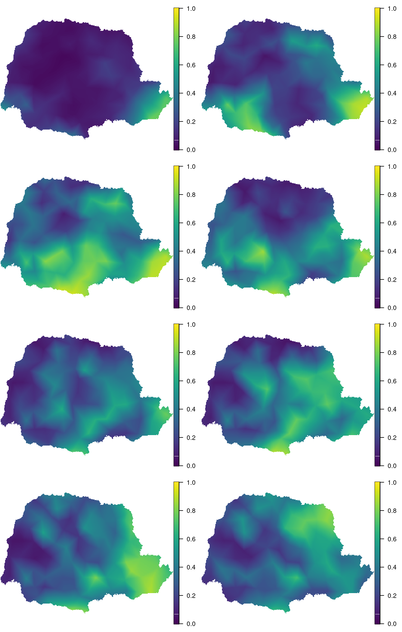
Figure 8.9: Posterior mean of the probability of rain at each time knot. Time flows from top to bottom and left to right.
References
Assunção, J. J., D. Gamerman, and R. M. Assunção. 1999. “Regional Differences in Factor Productivities of Brazilian Agriculture: A Space-Varying Parameter Approach.” Universidade Federal do Rio de Janeiro, Statistical Laboratory.
Assunção, R. M., J. E. Potter, and S. M. Cavenaghi. 2002. “A Bayesian Space Varying Parameter Model Applied to Estimating Fertility Schedules.” Statistics in Medicine 21: 2057–75.
Bailey, T. C., and A. C. Gatrell. 1995. Interactive Spatial Data Analysis. Harlow, UK: Longman Scientific & Technical.
Bowman, A. W., I. Gibson, E. M. Scott, and E. Crawford. 2010. “Interactive Teaching Tools for Spatial Sampling.” Journal of Statistical Software 36 (13): 1–17. http://www.jstatsoft.org/v36/i13/.
Cameletti, M., F. Lindgren, D. Simpson, and H. Rue. 2013. “Spatio-Temporal Modeling of Particulate Matter Concentration Through the Spde Approach.” Advances in Statistical Analysis 97 (2): 109–31.
Fuglstad, G-A., D. Simpson, F. Lindgren, and H. Rue. 2018. “Constructing Priors That Penalize the Complexity of Gaussian Random Fields.” Journal of the American Statistical Association to appear. https://doi.org/10.1080/01621459.2017.1415907.
Gamerman, D., A. R. B. Moreira, and H. Rue. 2003. “Space-Varying Regression Models: Specifications and Simulation.” Computational Statistics & Data Analysis - Special Issue: Computational Econometrics 42 (3): 513–33.
Gelfand, A. E., H-J Kim, C. F. Sirmans, and S. Banerjee. 2003. “Spatial Modeling with Spatially Varying Coefficient Processes.” Journal of the American Statistical Association 98 (462): 387–96.
Knorr-Held, L., and H. Rue. 2002. “On Block Updating in Markov Random Field Models for Disease Mapping.” Scandinavian Journal of Statistics 20: 597–614.
Petris, G., S. Petroni, and P. Campagnoli. 2009. Dynamic Linear Models with R. New York: Springer-Verlag.
Rowlingson, B. S., and P. J. Diggle. 1993. “Splancs: Spatial Point Pattern Analysis Code in S-Plus.” Computers & Geosciences 19 (5): 627–55. https://doi.org/https://doi.org/10.1016/0098-3004(93)90099-Q.
Rue, H., and L. Held. 2005. Gaussian Markov Random Fields: Theory and Applications. Monographs on Statistics & Applied Probability. Boca Raton, FL: Chapman & Hall.
Ruiz-Cárdenas, R., E. T. Krainski, and H. Rue. 2012. “Direct Fitting of Dynamic Models Using Integrated Nested Laplace Approximations — INLA.” Computational Statistics & Data Analysis 56 (6): 1808–28. https://doi.org/http://dx.doi.org/10.1016/j.csda.2011.10.024.
Simpson, D. P., J. B. Illian, F. Lindren, S. H Sørbye, and H. Rue. 2016. “Going Off Grid: Computationally Efficient Inference for Log-Gaussian Cox Processes.” Biometrika 103 (1): 49–70.
Simpson, D. P., H. Rue, A. Riebler, T. G. Martins, and S. H. Sørbye. 2017. “Penalising Model Component Complexity: A Principled, Practical Approach to Constructing Priors.” Statistical Science 32 (1): 1–28.
Taylor, B. M., T. M. Davies, Rowlingson B. S., and P. J. Diggle. 2013. “lgcp: An R Package for Inference with Spatial and Spatio-Temporal Log-Gaussian Cox Processes.” Journal of Statistical Software 52 (4): 1–40. http://www.jstatsoft.org/v52/i04/.
Vivar, J. C., and M. A. R. Ferreira. 2009. “Spatiotemporal Models for Gaussian Areal Data.” Journal of Computational and Graphical Statistics 18 (3): 658–74.
West, M., and J. Harrison. 1997. Bayesian Forecasting and Dynamic Models. New York: Springer-Verlag.