Chapter 4 Point processes and preferential sampling

4.1 Introduction

A point pattern records the occurrence of events in a study region. Typical examples include the locations of trees in a forest or the GPS coordinates of disease cases in a region. The locations of the observed events depend on an underlying spatial process, which is often modeled using an intensity function \(\lambda(\mathbf{s})\). The intensity function measures the average number of events per unit of space, and it can be modeled to depend on covariates and other effects. See Diggle (2014) or Baddeley, Rubak, and Turner (2015) for a recent summary on the analysis of spatial and spatio-temporal point patterns.

Under the log-Cox point process model assumption, we model the log intensity of the Cox process with a Gaussian linear predictor. In this case, the log-Cox process is known as a log-Gaussian Cox process (LGCP, Møller, Syversveen, and Waagepetersen 1998), and inference can be made using INLA. A Cox process is just a name for a Poisson process with varying intensity; thus we use the Poisson likelihood. The original approach that was used to fit these models in INLA (and other software) divides the study region into cells, which form a lattice, and counts the number of points in each one (Møller and Waagepetersen 2003). These counts can be modeled using a Poisson likelihood conditional on a Gaussian linear predictor and INLA can be used to fit the model (Illian, Sørbye, and Rue 2012). This can be done with the techniques already shown in this book.

In this chapter we focus on a new approach considering SPDE models directly, developed in Simpson et al. (2016). This approach has a nice theoretical justification and considers a direct approximation of the log-Cox point process model likelihood. Observations are modeled considering its exact location instead of binning them into cells. Along with the flexibility for defining a mesh, this approach can handle non-rectangular areas without wasting computational effort on a large rectangular area.

4.1.1 Definition of the LGCP

The Cox process is a Poisson process with intensity \(\lambda(\mathbf{s})\) that varies in space. Given some area \(A\) (for example a grid cell), the probability of observing a certain number of points in that area follows a Poisson distribution with intensity (expected value)

\[ \lambda_A = \int_A \lambda(\mathbf{s}) \ d\mathbf{s}. \]

The log-Gaussian part of the LGCP name comes from modeling \(\log(\lambda(\mathbf{s}))\) as a latent Gaussian (conditional on a set of hyper-parameters), in the typical GLM/GAM framework.

4.1.2 Data simulation

Data simulated here will be used later in Section 4.2 and Section 4.3. To sample from a log-Cox point process the function used is rLGCP() from the spatstat package (Baddeley, Rubak, and Turner 2015). We use a \((0,3) \times (0,3)\) simulation window. In order to define this window using function owin() (in package spatstat):

library(spatstat)
win <- owin(c(0, 3), c(0, 3))

The rLGCP function uses the GaussRF() function, in package RandomFields (Schlather et al. 2015), to simulate from the spatial field over a grid. There is an internal parameter to control the resolution of the grid, which we specify to give 300 pixels in each direction:

npix <- 300
spatstat.options(npixel = npix)

We model the intensity as

\[ \log(\lambda(\mathbf{s})) = \beta_0 + S(\mathbf{s}), \]

with \(\beta_0\) a fixed value and \(S(\mathbf{s})\) a Gaussian spatial process with Matérn covariance and zero mean. Parameter \(\beta_0\) can be regarded as a global mean level for the log intensity; i.e. the log-intensity fluctuates about it according to the spatial process \(S(\mathbf{s})\).

If there is no spatial field, the expected number of points is \(e^{\beta_0}\) times the area of the window. This means that the expected number of points is:

beta0 <- 3
exp(beta0) * diff(range(win$x)) * diff(range(win$y))
## [1] 180.8

Hence, this value of beta0 will produce a reasonable number of points in the following simulations. If we set beta0 too small, we will get almost no points, and we would not be able to produce reasonable results. It is also possible to use a function on several covariates, e.g. a GLM (see Section 4.2).

In this chapter we use a Matérn covariance function with \(\nu = 1\). The other parameters are the variance and scale. The following values for these parameters will produce a smooth intensity of the point process:

sigma2x <- 0.2
range <- 1.2
nu <- 1

The value of sigma2x is set to make the log-intensity vary a bit around the mean, but always within a reasonable range of values. Furthermore, with these parameters \(\nu = 1\) and the range of the spatial process \(S(\mathbf{s})\) is (about) 2, which produces smooth changes in the current study window. Smaller values of the practical range will produce a spatial process \(S(s)\) (and, in turn the intensity of the spatial process) that changes rapidly over the study window. Similarly, very large values of the practical range will produce an almost constant spatial process \(S(s)\), so that the log-intensity will be very close to \(\beta_0\) at all points of the study window.

The points of the point process are simulated as follows:

library(RandomFields)
set.seed(1)
lg.s <- rLGCP('matern', beta0, var = sigma2x,
  scale = range / sqrt(8), nu = nu, win = win)

Both the spatial field and the point pattern are returned. The coordinates of the observed events of the point pattern can be obtained as follows:

xy <- cbind(lg.s$x, lg.s$y)[, 2:1]

The number of simulated points is:

(n <- nrow(xy))
## [1] 217

The exponential of the simulated values of the spatial field are returned as the Lambda attribute of the object. Below, we extract the values of \(\lambda (\mathbf{s})\) and summarize the \(\log(\lambda(\mathbf{s}))\).

Lam <- attr(lg.s, 'Lambda')
rf.s <- log(Lam$v)
summary(as.vector(rf.s))
##    Min. 1st Qu.  Median    Mean 3rd Qu.    Max. 
##    2.33    2.91    3.13    3.15    3.37    4.47

Figure 4.1 shows the simulated spatial field and the point pattern.

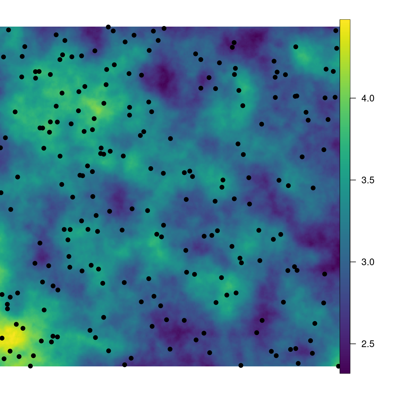
Figure 4.1: Simulated intensity of the point process and simulated point pattern (black dots).

4.1.3 Inference

Following Simpson et al. (2016), the parameters of the log-Gaussian Cox point process model can be estimated with INLA. In simplified terms, we will construct an augmented dataset and run a Poisson regression with INLA. The augmented data set is made of a binary response, with 1 for the observed points and 0 for some dummy observations. Both the observed and dummy observations will have associated ‘expected values’ or weights that will be included in the Poisson regression. This will be explained step by step in the following sections.

4.1.3.1 The mesh and the weights

For appropriate inference with the LGCP, we must take some care when building the mesh. In the particular case of the analysis of point patterns, we do not usually use the location points as mesh nodes. We need a mesh that covers the study region; for this we use the loc.domain to build the mesh. Further, we only use a small first outer extension, but no second outer extension.

loc.d <- 3 * cbind(c(0, 1, 1, 0, 0), c(0, 0, 1, 1, 0))
mesh <- inla.mesh.2d(loc.domain = loc.d, offset = c(0.3, 1), 
  max.edge = c(0.3, 0.7), cutoff = 0.05)
nv <- mesh$n

This mesh can be seen in Figure 4.2.

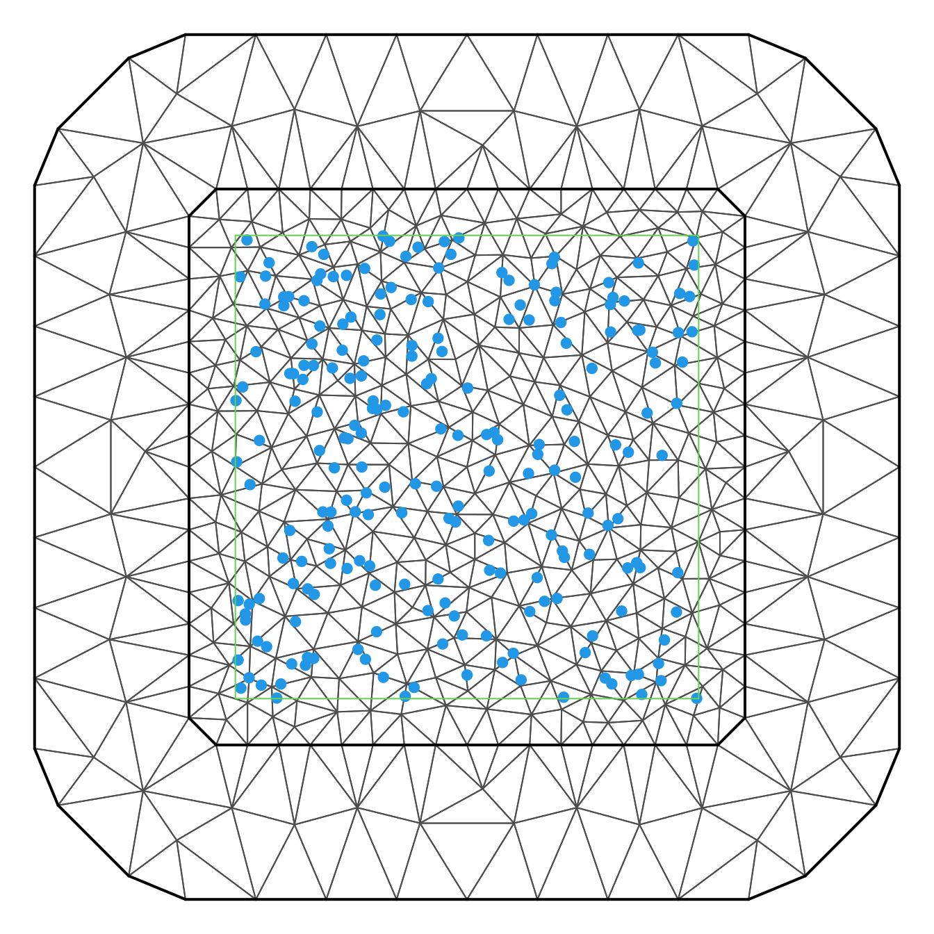
Figure 4.2: Mesh used to fit a log-Gaussian Cox process to a point pattern.

The SPDE model will be defined considering the PC-priors derived in Fuglstad et al. (2018) for the model parameters range and marginal standard deviation. These are defined as follows:

spde <- inla.spde2.pcmatern(mesh = mesh,
  # PC-prior on range: P(practic.range < 0.05) = 0.01
  prior.range = c(0.05, 0.01),
  # PC-prior on sigma: P(sigma > 1) = 0.01
  prior.sigma = c(1, 0.01)) 

The SPDE approach for point pattern analysis defines the model at the nodes of the mesh. To fit the log-Cox point process model, these points are considered as integration points. The method in Simpson et al. (2016) defines the expected number of events to be proportional to the area around the node (the areas of the polygons in the dual mesh). This means that at the nodes of the mesh with larger triangles, there are also larger expected values. inla.mesh.fem(mesh)$va gives this value for every mesh node. These values for the nodes in the inner domain can be used to compute the intersection between the dual mesh polygons and the study domain polygon. To do that, we use the function book.mesh.dual():

dmesh <- book.mesh.dual(mesh)

This function is available in the file spde-book-functions.R, and it returns the dual mesh in an object of class SpatialPolygons. We have plotted the dual mesh in Figure 4.3.

The domain polygon can be converted into a SpatialPolygons class as follows:

domain.polys <- Polygons(list(Polygon(loc.d)), '0')
domainSP <- SpatialPolygons(list(domain.polys))

Because the mesh is larger than the study area, we need to compute the intersection between each polygon in the dual mesh and the study area:

library(rgeos)
w <- sapply(1:length(dmesh), function(i) {
  if (gIntersects(dmesh[i, ], domainSP))
    return(gArea(gIntersection(dmesh[i, ], domainSP)))
  else return(0)
})

The sum of these weights is the area of the study region:

sum(w)
## [1] 9

We can also check how many integration points have zero weight:

table(w > 0)
## 
## FALSE  TRUE 
##   197   288

The integration points with zero weight are identified in red in Figure 4.3. Note how all of them, and the associated polygons, are outside the study region.

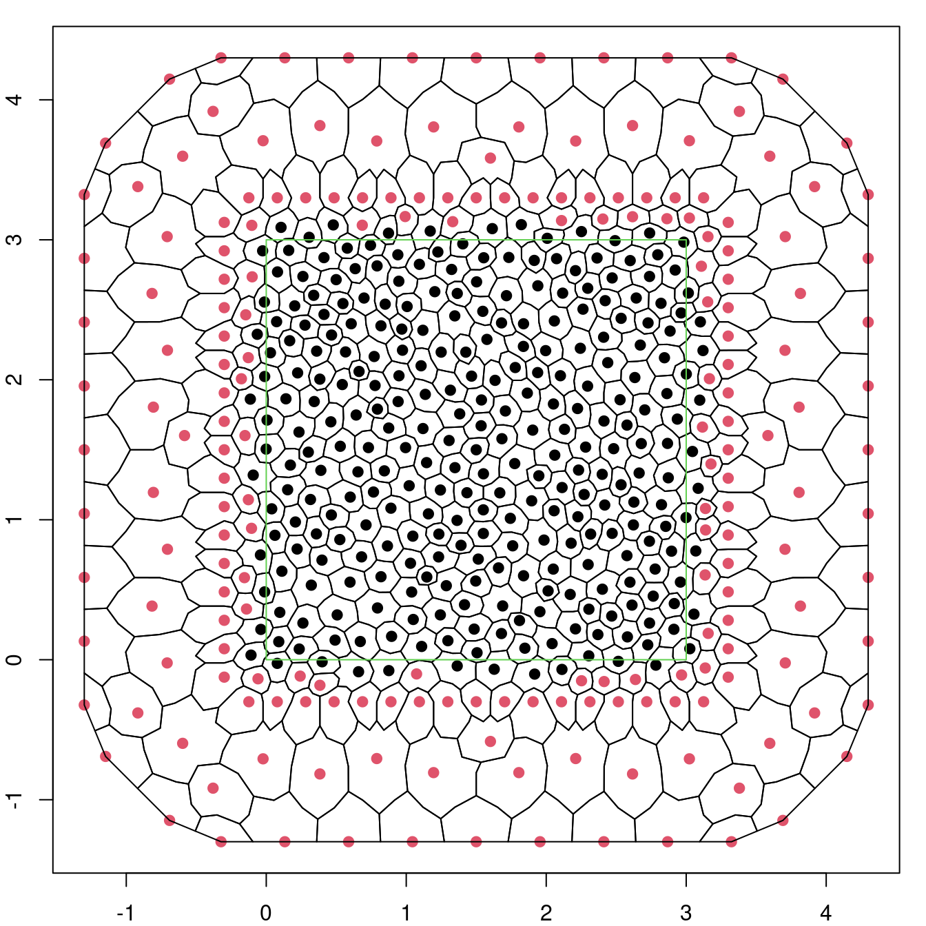
Figure 4.3: Voronoy polygons for the mesh used to make inference for the log-Gaussian Cox process.

4.1.3.2 Data and projection matrices

The vector of weights we have computed is exactly what we need to use as the exposure (E) in the Poisson likelihood in INLA (with the minor modification that \(\log(E)\) is defined as zero if \(E=0\)). We augment the vector of ones for the observations (representing the points) with a sequence of zeros (representing the mesh nodes):

y.pp <- rep(0:1, c(nv, n))

The exposure vector can be defined as:

e.pp <- c(w, rep(0, n)) 

The projection matrix is defined in two steps. For the integration points this is just a diagonal matrix because these locations are just the mesh vertices:

imat <- Diagonal(nv, rep(1, nv))

For the observed points, another projection matrix is defined:

lmat <- inla.spde.make.A(mesh, xy)

The entire projection matrix is:

A.pp <- rbind(imat, lmat)

We set up the data stack as follows:

stk.pp <- inla.stack(
  data = list(y = y.pp, e = e.pp), 
  A = list(1, A.pp),
  effects = list(list(b0 = rep(1, nv + n)), list(i = 1:nv)),
  tag = 'pp')

4.1.3.3 Posterior marginals

The posterior marginals for all parameters of the model are obtained by fitting the model with INLA:

pp.res <- inla(y ~ 0 + b0 + f(i, model = spde), 
  family = 'poisson', data = inla.stack.data(stk.pp), 
  control.predictor = list(A = inla.stack.A(stk.pp)), 
  E = inla.stack.data(stk.pp)$e)

The summary for the model hyperparameters, i.e., range and standard deviation of the spatial field, is:

pp.res$summary.hyperpar
##               mean     sd 0.025quant 0.5quant 0.975quant
## Range for i 0.5947 1.0502    0.06651   0.3050      2.907
## Stdev for i 0.0741 0.0533    0.00962   0.0618      0.209
##               mode
## Range for i 0.1367
## Stdev for i 0.0291

The posterior marginal distributions of the log-Gaussian Cox model parameters are displayed in Figure 4.4.

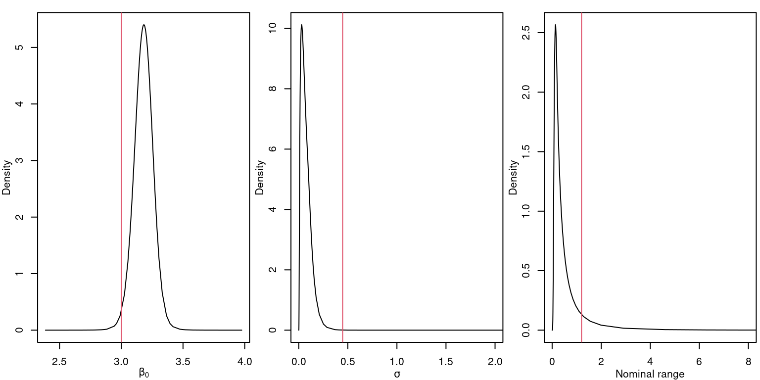
Figure 4.4: Posterior distribution for the parameters of the log-Gaussian Cox model \(\beta_0\) (left), \(\sigma\) (center) and the nominal range (right). Vertical lines represent the actual values of the parameters.

4.2 Including a covariate in the log-Gaussian Cox process

In this section we add a covariate to the linear predictor in the log-Gaussian Cox model. To approximate the Cox likelihood well, we need the covariate to vary slowly in space; i.e. it should not change much between neighboring mesh nodes. For model fitting, we must know the value of the covariate at the location points and integration points.

4.2.1 Simulation of the covariate

First, we define a covariate everywhere in the study area, as

\[ f(s_1, s_2) = \cos(s_1) - \sin(s_2 - 2). \]

This function will be computed at a grid defined from the settings in the spatstat package (e.g., the number of pixels in each direction). The locations where we simulate cover both the study window and the mesh points, as values of the covariate are required for both types of points:

# Use expanded range
x0 <- seq(min(mesh$loc[, 1]), max(mesh$loc[, 1]), length = npix)
y0 <- seq(min(mesh$loc[, 2]), max(mesh$loc[, 2]), length = npix)
gridcov <- outer(x0, y0, function(x,y) cos(x) - sin(y - 2))

Now, the expected number of points is a function of the covariate:

beta1 <- -0.5
sum(exp(beta0 + beta1 * gridcov) * diff(x0[1:2]) * diff(y0[1:2]))
## [1] 702.6

We simulate the point pattern using:

set.seed(1)
lg.s.c <- rLGCP('matern', im(beta0 + beta1 * gridcov, xcol = x0,
  yrow = y0), var = sigma2x, scale = range / sqrt(8), 
  nu = 1, win = win)

Both the spatial field and the point pattern are returned. The point pattern locations are:

xy.c <- cbind(lg.s.c$x, lg.s.c$y)[, 2:1]
n.c <- nrow(xy.c)

The values of the simulated covariate and the simulated spatial field over the grid can be seen in Figure 4.5.

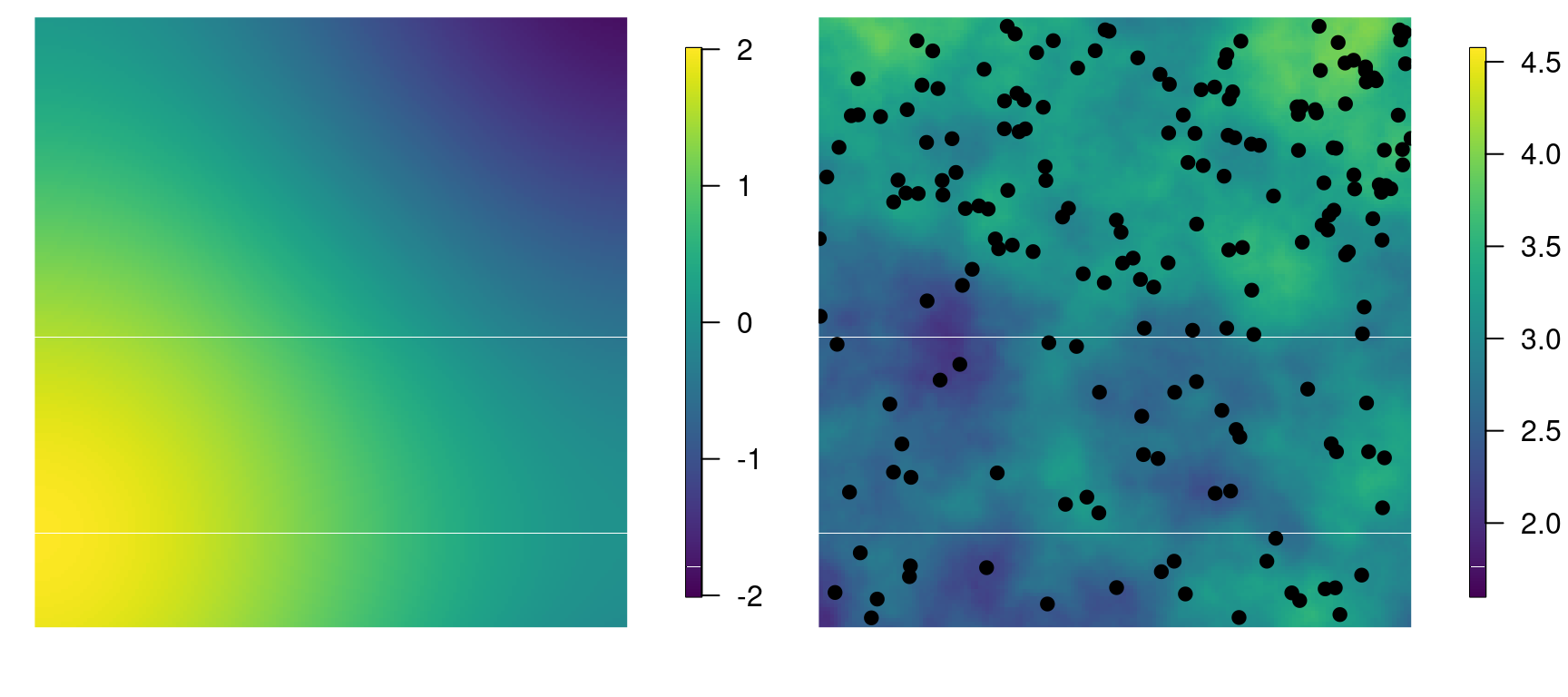
Figure 4.5: Simulated covariate (left) and simulated log-intensity of the point process, along with the simulated point pattern (right).

4.2.2 Inference

The covariate values need to be included in the data and the model for inference. These values must be available at the point pattern locations and at the mesh nodes. These values can be collected by interpolating from the grid data (in an im object) using function interp.im():

covariate.im <- im(gridcov, x0, y0)
covariate <- interp.im(covariate.im, 
  x = c(mesh$loc[, 1], xy.c[, 1]),
  y = c(mesh$loc[, 2], xy.c[, 2]))

The augmented data is created in the same way as before:

y.pp.c <- rep(0:1, c(nv, n.c))
e.pp.c <- c(w, rep(0, n.c))

The projection matrix for the observed locations is:

lmat.c <- inla.spde.make.A(mesh, xy.c)

The two projection matrices can be merged with rbind() into a total projection matrix for the augmented data:

A.pp.c <- rbind(imat, lmat.c)

The data stack now includes the covariates, but is otherwise the same as in Section 4.1.3.2:

stk.pp.c <- inla.stack(
  data = list(y = y.pp.c, e = e.pp.c), 
  A = list(1, A.pp.c), 
  effects = list(list(b0 = 1, covariate = covariate), 
    list(i = 1:nv)),
  tag = 'pp.c')

Finally, the model is fitted with the following R code:

pp.c.res <- inla(y ~ 0 + b0 + covariate + f(i, model = spde),
  family = 'poisson', data = inla.stack.data(stk.pp.c), 
  control.predictor = list(A = inla.stack.A(stk.pp.c)), 
  E = inla.stack.data(stk.pp.c)$e)

A summary of the model hyperparameters is given below.

pp.c.res$summary.hyperpar
##               mean     sd 0.025quant 0.5quant 0.975quant
## Range for i 0.9611 2.4193    0.08109   0.3928      5.332
## Stdev for i 0.0774 0.0542    0.00946   0.0656      0.208
##               mode
## Range for i 0.1553
## Stdev for i 0.0291

The posterior distributions of the log-Gaussian Cox model parameters are shown in Figure 4.6.

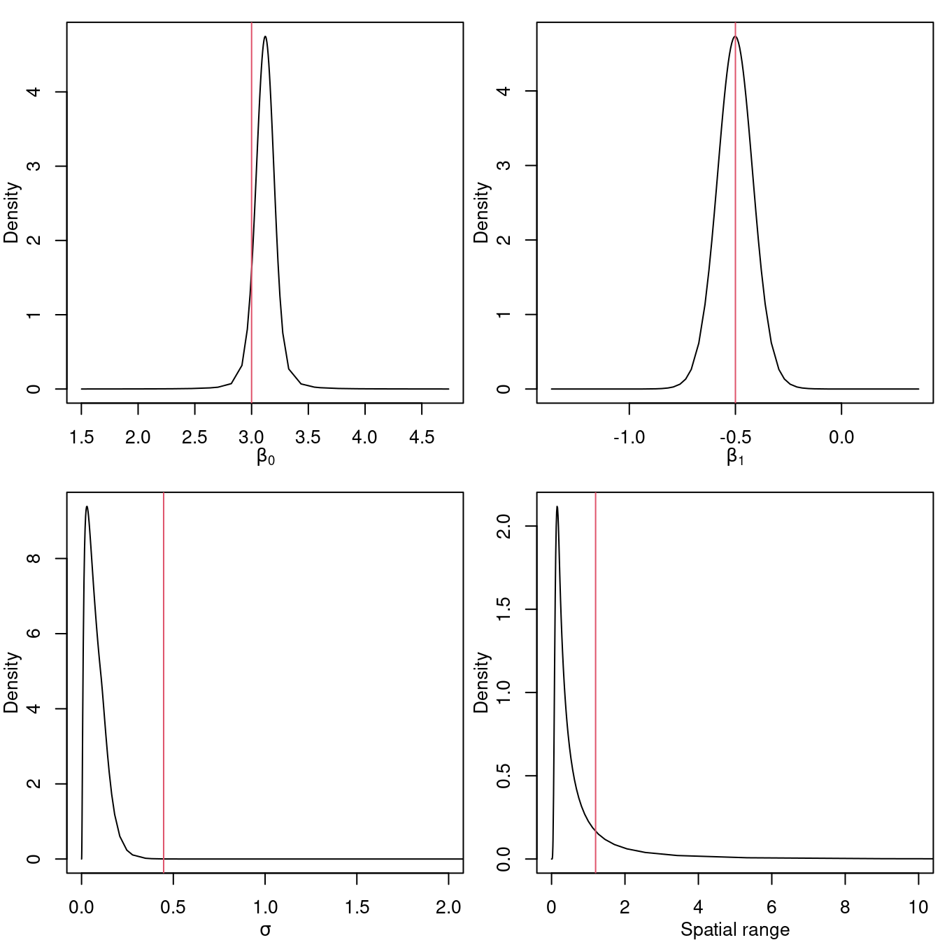
Figure 4.6: Posterior distribution for the intercept (top left), coefficient of the covariate (top right) and the parameters of the log-Cox model \(\sigma\) (bottom left) and nominal range (bottom right). Vertical lines represent the actual values of the parameters.

4.3 Geostatistical inference under preferential sampling

In some cases, the sampling effort depends on the response (the marks or observed values at the points). For example, it is more common to have stations collecting data about pollution in industrial areas than in rural ones. This type of sampling is called preferential sampling. To make inference in this case, it is necessary to test whether there is a preferential sampling problem with our data. One approach is to build a joint model considering a log-Gaussian Cox model for the point pattern (the locations) and the response (Diggle, Menezes, and Su 2010). Hence, inference on a joint model is required in this case.

This approach assumes a linear predictor for the point process as:

\[ \eta_i^{pp} = \beta_0^{pp} + u_i. \]

For the observations, the linear predictor is a function of the latent Gaussian random field for the point process:

\[ \eta_i^{y} = \beta_0^{y} + \beta u_i \]

where \(\beta_0^y\) is an intercept for the observations and \(\beta\) is a weight on the shared random field effect.

An illustration of the use of INLA for the preferential sampling problem is available at http://www.r-inla.org/examples/case-studies/diggle09 in the R-INLA web page. The example therein uses a two dimensional random walk model for the latent random field. Here, the model considers geostatistical inference under preferential sampling using SPDE.

To simulate this joint likelihood we have to use the same underlying spatial field when simulating the point pattern and when simulating the observations. The \(y\)-values assigned to a point pattern location will use the value of the random field at the nearest grid point. The values of the spatial field are collected at the closest grid centers as follows:

z <- log(t(Lam$v)[do.call('cbind',
  nearest.pixel(xy[, 1], xy[, 2], Lam))])

We summarize these values:

summary(z)
##    Min. 1st Qu.  Median    Mean 3rd Qu.    Max. 
##    2.49    2.96    3.24    3.24    3.50    4.42

These values are the latent field with zero mean plus the defined intercept \(\beta_0^{pp}\). The response (the marks) is defined to have a different intercept \(\beta_0^y\) plus the zero mean random field multiplied by \(1/\beta\), where \(\beta\) is the weight on the shared random field between the intensity of the point process locations and the response. Then, the response is simulated as follows:

beta0.y <- 10
beta <- -2
prec.y <- 16

set.seed(2)
resp <- beta0.y + (z - beta0) / beta + 
  rnorm(length(z), 0, sqrt(1 / prec.y))

A summary of the simulated values of the response is below:

summary(resp)
##    Min. 1st Qu.  Median    Mean 3rd Qu.    Max. 
##    9.08    9.66    9.91    9.88   10.09   10.60

As \(\beta < 0\), the response values are lower where we have more observation locations. In a real data application this might be the case if there is a preference for survey locations where low values are expected.

4.3.1 Fitting the usual model

Here, a geostatistical model is fitted using the usual approach; i.e., the locations are considered as fixed. The mesh used to define the SPDE model is the same one as in the previous section. Hence, the data stack and the model can be fitted as follows:

stk.u <- inla.stack(
  data = list(y = resp),
  A = list(lmat, 1), 
  effects = list(i = 1:nv, b0 = rep(1, length(resp))))

u.res <- inla(y ~ 0 + b0 + f(i, model = spde),
  data = inla.stack.data(stk.u), 
  control.predictor = list(A = inla.stack.A(stk.u)))

A summary of the estimated values of the model parameters and the true values used to simulate the data are in Table 4.1. There, \(1/\sigma^2_y\) denotes the precision of the Gaussian observations.

Table 4.1: Posterior modes of some of the model parameters.

Parameter	True	Mean	St. Dev.	2.5% quant.	97.5% quant.
\(\beta_0^y\)	10	9.884	0.1105	9.629	10.10
\(1/\sigma^2_y\)	16	12.462	1.3590	9.899	15.22

In addition, the posterior distribution marginals of the model parameters are in Figure 4.7.

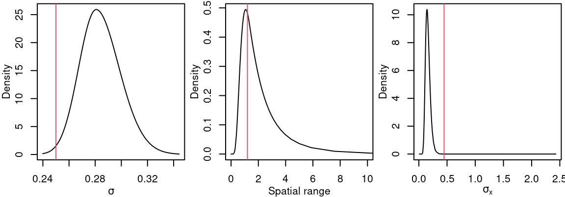
Figure 4.7: Posterior distribution for \(\sigma\), the range and standard deviation of the spatial effect just using the response. Vertical lines represent the actual values of the parameters.

4.3.2 Model fitting under preferential sampling

Under preferential sampling, the fitted model is defined so that a LGRF is considered to model both point pattern and the response. Using INLA this can be done using two likelihoods: one for the point pattern and another one for the response. To do it, data must include a matrix response and a new index set to specify the model for the LGRF. This can be easily done by using the inla.stack() function following previous examples for models with two likelihoods.

The point pattern ‘observations’ are put in the first column and the response values in the second column. So, the data stack is redefined for the response and the point process. The response will be in the first column and the Poisson data for the point process in the second column. Also, to avoid the expected number of cases as NA for the Poisson likelihood, it is set as zero in the response part of the data stack. The SPDE effect in the point process part is modeled as a copy of the SPDE effect in the response part. This is done by defining an index set with a different name and using it in the copy feature later. See the code below.

stk2.y <- inla.stack(
  data = list(y = cbind(resp, NA), e = rep(0, n)), 
  A = list(lmat, 1),
  effects = list(i = 1:nv, b0.y = rep(1, n)),
  tag = 'resp2')

stk2.pp <- inla.stack(data = list(y = cbind(NA, y.pp), e = e.pp), 
  A = list(A.pp, 1),
  effects = list(j = 1:nv, b0.pp = rep(1, nv + n)),
  tag = 'pp2')

j.stk <- inla.stack(stk2.y, stk2.pp)

Now, the geostatistical model is fitted under preferential sampling. To include the LGRF in both likelihoods, the copy effect in INLA is used. We assign a \(N(0, 2^{-1})\) prior for this parameter as follows:

# Gaussian prior
gaus.prior <- list(prior = 'gaussian', param = c(0, 2))
# Model formula
jform <- y ~ 0 + b0.pp + b0.y + f(i, model = spde) +
  f(j, copy = 'i', fixed = FALSE,
    hyper = list(beta = gaus.prior))
# Fit model
j.res <- inla(jform, family = c('gaussian', 'poisson'), 
  data = inla.stack.data(j.stk),
  E = inla.stack.data(j.stk)$e,
  control.predictor = list(A = inla.stack.A(j.stk)))

Values of the parameters used in the simulation of the data and a summary of their posterior distributions are shown in Table 4.2.

Table 4.2: Posterior modes of some of the model parameters under preferential sampling.

Parameter	True	Mean	St. Dev.	2.5% quant.	97.5% quant.
\(\beta_0\)	3	3.204	0.1575	2.908	3.545
\(\beta_0^y\)	10	9.883	0.1217	9.612	10.120

Posterior marginal distributions for the model parameters from the result considering only the point process (PP), only the observations/marks (\(\mathbf{Y}\)) and jointly are in Figure 4.8. Notice that for the \(\beta_0\) parameter there are results considering only the PP and joint, for \(\beta_0^y\) the results are only for \(\mathbf{Y}\) and the joint model, and for \(\beta\) (fitted using copy) the results are only from the joint model. Results from the three models are only available for the random field parameters.

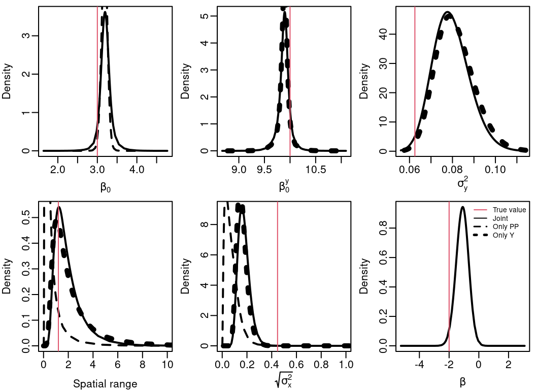
Figure 4.8: Posterior marginal distribution for the intercept for the point process \(\beta_0\), intercept for the observations \(\beta_0^y\), noise variance in the observations \(\sigma^2_y\), the practical range, the marginal standard deviation for the random field \(\sigma^2_x\) and the sharing coefficient \(\beta\).

References

Baddeley, A., E. Rubak, and R. Turner. 2015. Spatial Point Patterns: Methodology and Applications with R. Boca Raton, FL: Chapman & Hall/CRC.

Diggle, P. 2014. Statistical Analysis of Spatial and Spatio-Temporal Point Patterns. 3rd ed. Boca Raton, FL: CRC Press, Taylor & Francis Group.

Diggle, P. J., R. Menezes, and T-L. Su. 2010. “Geostatistical Inference Under Preferential Sampling.” Journal of the Royal Statistical Society: Series C (Applied Statistics) 59 (2): 191–232. https://doi.org/10.1111/j.1467-9876.2009.00701.x.

Fuglstad, G-A., D. Simpson, F. Lindgren, and H. Rue. 2018. “Constructing Priors That Penalize the Complexity of Gaussian Random Fields.” Journal of the American Statistical Association to appear. https://doi.org/10.1080/01621459.2017.1415907.

Illian, J. B., S. H. Sørbye, and H. Rue. 2012. “A Toolbox for Fitting Complex Spatial Point Process Models Using Integrated Nested Laplace Approximation (INLA).” Annals of Applied Statistics 6 (4): 1499–1530.

Møller, J., A. R. Syversveen, and R. P. Waagepetersen. 1998. “Log Gaussian Cox Processes.” Scandinavian Journal of Statistics 25: 451–82.

Møller, J., and R. P. Waagepetersen. 2003. Statistical Inference and Simulation for Spatial Point Processes. Boca Raton, FL: Chapman & Hall/CRC.

Schlather, Martin, Alexander Malinowski, Peter J. Menck, Marco Oesting, and Kirstin Strokorb. 2015. “Analysis, Simulation and Prediction of Multivariate Random Fields with Package RandomFields.” Journal of Statistical Software 63 (8): 1–25. http://www.jstatsoft.org/v63/i08/.

Simpson, D. P., J. B. Illian, F. Lindren, S. H Sørbye, and H. Rue. 2016. “Going Off Grid: Computationally Efficient Inference for Log-Gaussian Cox Processes.” Biometrika 103 (1): 49–70.