Chapter 7 Space-time models
In this chapter we detail how to fit separable space-time models. A separable space-time model is defined as a SPDE model for the spatial domain and an autoregressive model of order 1, i.e., AR(\(1\)), for the time dimension. The space-time separable model is defined by the Kronecker product between the precision matrices of the spatial and temporal random effects. Additional information about separable space-time models can be found in Cameletti et al. (2013).
In this chapter we start by showing two different ways to implement space-time models. The first one uses discrete time domain and the second one considers continuous time and discretizes this over a set of knots. The main difference in the model fitting process is that when we use continuous time, we need to choose time knots and to adjust the projector matrix to use these knots. However, none of the approaches requires the measurement locations to be the same over time.
In this chapter we focus on basic code examples, together with information on how to structure the models for faster computation. In the following chapter we will provide several advanced examples.
7.1 Discrete time domain
In this section we show how to fit a space-time separable model, as in Cameletti et al. (2013). Additionally, we show how to include a categorical covariate.
7.1.1 Data simulation
The study region considered in this example is the border of Paraná state,
available in package INLA, as in Section 2.8. This boundary
will be used as the domain of the spatial process and it can be loaded as:
data(PRborder)The first step is to define the spatial model. To be able to fit the model quickly, we use the low resolution mesh for Paraná state border created in Section 2.6.
There are two options to simulate from the model proposed in Cameletti et al. (2013). The first one is based on the simultaneous distribution of the latent field and the second one is based on the conditional simulation at each time. This last option is easy to compute as each time point is simulated conditionally on the previous one, giving linear run time for long temporal simulations.
First, the time dimension is set to \(k=12\):
k <- 12The locations of the points are the same as in
dataset PRprec, but considered
in a randomized order:
data(PRprec)
coords <- as.matrix(PRprec[sample(1:nrow(PRprec)), 1:2])
In the following simulation step we will use the book.rspde()
function available in the file spde-book-functions.R.
The \(k\) independent realizations of the spatial model can be generated as follows:
params <- c(variance = 1, kappa = 1)

set.seed(1)
x.k <- book.rspde(coords, range = sqrt(8) / params[2],
  sigma = sqrt(params[1]), n = k, mesh = prmesh1,
  return.attributes = TRUE)
The number of space-time observations is the number of rows of x.k and it
can be checked with:
dim(x.k)
## [1] 616  12
Now, the autoregressive parameter \(\rho\) for the temporal effect is defined:
rho <- 0.7Next, temporal correlation is introduced:
x <- x.k
for (j in 2:k)
  x[, j] <- rho * x[, j - 1] + sqrt(1 - rho^2) * x.k[, j]
Here, the \(\sqrt{1-\rho^2}\) term is added to make the process stationary in time, see Rue and Held (2005) and Cameletti et al. (2013). Figure 7.1 shows the realization of the space-time process.
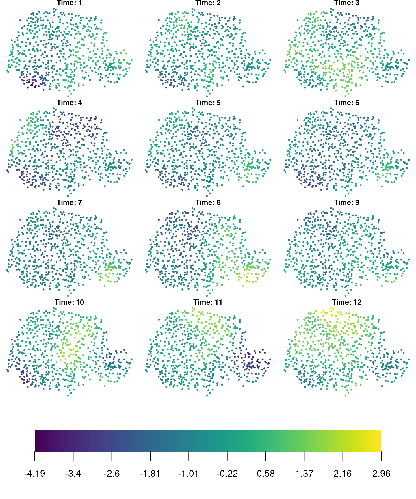
Figure 7.1: Realization of the space-time random field.
In this example, a categorical covariate will be included in the model. We
simulate a categorical covariate with three levels (labeled A, B and C):
n <- nrow(coords)
set.seed(2)
ccov <- factor(sample(LETTERS[1:3], n * k, replace = TRUE))
The distribution of values of this categorical covariate is:
table(ccov)
## ccov
##    A    B    C
## 2469 2441 2482
The regression coefficients and the regression parameters are:
beta <- -1:1The response variable will be computed by adding the fixed effect on the categorical covariate, the spatio-temporal random effect and some random white noise (with standard deviation 0.1):
sd.y <- 0.1
y <- beta[unclass(ccov)] + x + rnorm(n * k, 0, sd.y)
The average value of the response on the levels of the categorical covariate are:
tapply(y, ccov, mean)
##       A       B       C
## -1.4112 -0.3998  0.6024
To show that we can use different locations at different times, some of the observations will be dropped. In particular, only half of the simulated data will be kept. This can be done by creating an index for the selected observations, as follows:
isel <- sample(1:(n * k), n * k / 2) These data are then put together in a data.frame:
dat <- data.frame(y = as.vector(y), w = ccov,
  time = rep(1:k, each = n),
  xcoo = rep(coords[, 1], k),
  ycoo = rep(coords[, 2], k))[isel, ]
In real applications there may be completely misaligned locations across different times. The code we provide in this example will work in that situation.
7.1.2 Data stack preparation
We use the PC-priors derived in Fuglstad et al. (2018) for the model parameters range and marginal standard deviation. These are set when defining the SPDE, as follows:
spde <- inla.spde2.pcmatern(mesh = prmesh1,
  prior.range = c(0.5, 0.01), # P(range < 0.05) = 0.01
  prior.sigma = c(1, 0.01)) # P(sigma > 1) = 0.01
Now, additional data preparation is required to build the space-time model. The index set is made taking into account the number of mesh points in the SPDE model and the number of groups, as:
iset <- inla.spde.make.index('i', n.spde = spde$n.spde,
  n.group = k)
Note that the index set for the latent field does not depend on the data set
locations. It only depends on the SPDE model size and on the time dimension.
The projection matrix is defined using the coordinates of the observed data. We
need to pass the time index to the group argument to build the projector
matrix and the inla.spde.make.A() function:
A <- inla.spde.make.A(mesh = prmesh1,
  loc = cbind(dat$xcoo, dat$ycoo), group = dat$time)
The effects in the stack is a list with two elements: the first one is the
index set and the second one the categorical covariate. The stack data is
defined as:
sdat <- inla.stack(
  data = list(y = dat$y),
  A = list(A, 1),
  effects = list(iset, w = dat$w),
  tag = 'stdata')
7.1.3 Fitting the model and some results
In this example, a PC-prior (see Section 1.6.5) is also used for the temporal autoregressive parameter, i.e., the autocorrelation parameter. In particular, this prior considers that \(P(cor>0)=0.9\) and it is defined as follows:
h.spec <- list(rho = list(prior = 'pc.cor1', param = c(0, 0.9)))To deal with the categorical covariate we need to use
expand.factor.strategy = 'inla' in the control.fixed argument list to get an intuitive result. Hence, model fitting is done as follows:
# Model formula
formulae <- y ~ 0 + w + f(i, model = spde, group = i.group,
  control.group = list(model = 'ar1', hyper = h.spec))
# PC prior on the autoreg. param.
prec.prior <- list(prior = 'pc.prec', param = c(1, 0.01))
# Model fitting
res <- inla(formulae,  data = inla.stack.data(sdat),
  control.predictor = list(compute = TRUE,
    A = inla.stack.A(sdat)),
  control.family = list(hyper = list(prec = prec.prior)),
  control.fixed = list(expand.factor.strategy = 'inla'))
A summary of the three intercepts, together with the observed mean for each covariate level, is:
cbind(Obs. = tapply(dat$y, dat$w, mean), res$summary.fixed[, -7])
##     Obs.   mean    sd 0.025quant 0.5quant 0.975quant   mode
## A -1.378 -1.280 0.406    -2.0814   -1.280     -0.476 -1.281
## B -0.420 -0.282 0.406    -1.0841   -0.283      0.521 -0.284
## C  0.614  0.720 0.406    -0.0814    0.720      1.524  0.719
The posterior marginal distributions for the random field parameters and the marginal distribution for the temporal correlation are displayed in Figure 7.2.
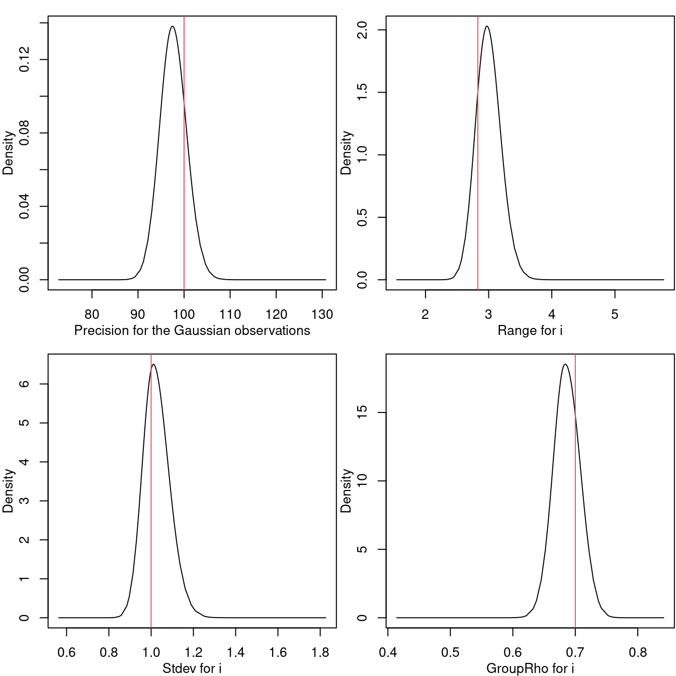
Figure 7.2: Marginal posterior distribution for the precision of the Gaussian likelihood (top-left), the practical range (top-right), standard deviation of the field (bottom-left) and the temporal correlation (bottom-right). The red vertical lines are placed at the true values of the parameters.
7.1.4 A look at the posterior random field
The random field posterior distribution can be compared to the realized random field by means of the posterior mean, median, mode or any other quantile.
Before we get to this point, we need the index for the random field at the data locations:
idat <- inla.stack.index(sdat, 'stdata')$dataThe correlation between the simulated data response and the posterior mean of the predicted values can be computed as follows:
cor(dat$y, res$summary.linear.predictor$mean[idat])
## [1] 0.998
The correlation is almost one because there is no error term in the model.
We now compute predictions for each time point. First, a grid is defined in the same way as in the rainfall example in Section 2.8:
stepsize <- 4 * 1 / 111
nxy <- round(c(diff(range(coords[, 1])),
  diff(range(coords[, 2]))) / stepsize)
projgrid <- inla.mesh.projector(
  prmesh1, xlim = range(coords[, 1]),
  ylim = range(coords[, 2]), dims = nxy)
Then, the prediction for each time can be done as follows:
xmean <- list()
for (j in 1:k)
  xmean[[j]] <- inla.mesh.project(
    projgrid, res$summary.random$i$mean[iset$i.group == j])
Next, we subset to the points of the grid inside the
boundaries of Paraná state, and set the points of the grid out of the Paraná border to NA:
library(splancs)
xy.in <- inout(projgrid$lattice$loc,
  cbind(PRborder[, 1], PRborder[, 2]))
We visualize the result in Figure 7.3.
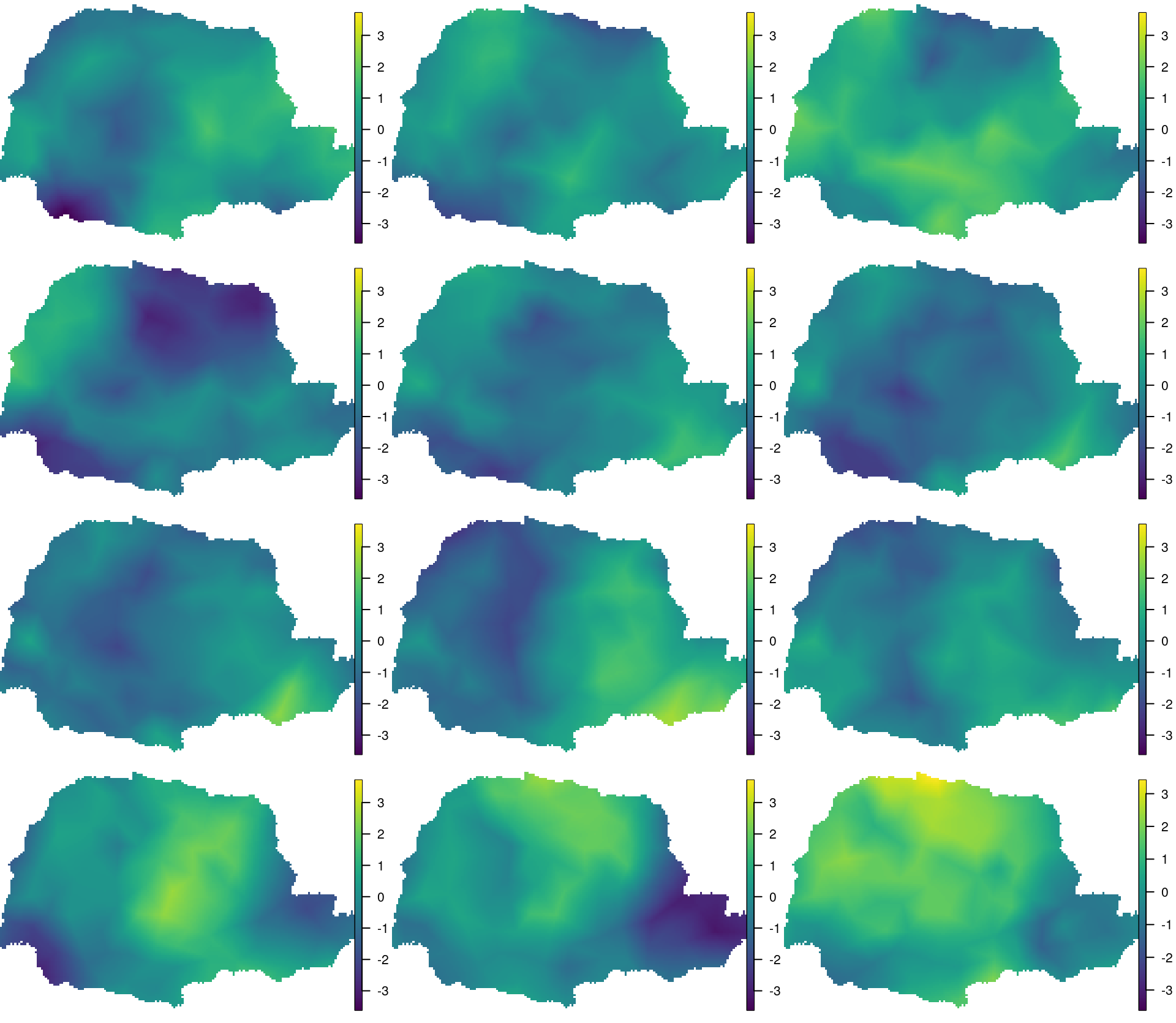
Figure 7.3: Visualization of the posterior mean of the space-time random field. Time flows from top to bottom and left to right.
7.1.5 Validation
The inference results we just showed are based only on part of the simulated data. The other part of the simulated data can now be used for validation. Therefore, another data stack is required to compute posterior distributions for the validation data:
vdat <- data.frame(r = as.vector(y), w = ccov,
  t = rep(1:k, each = n), x = rep(coords[, 1], k),
  y = rep(coords[, 2], k))
vdat <- vdat[-isel, ]
We compute a projection matrix and the data stack for the validation data:
Aval <- inla.spde.make.A(prmesh1,
  loc = cbind(vdat$x, vdat$y), group = vdat$t)
stval <- inla.stack(
  data = list(y = NA), # NA: no data, only enable predictions
  A = list(Aval, 1),
  effects = list(iset, w = vdat$w),
  tag = 'stval')
Next, we join these two stacks together into a full stack and re-fit the model. We use the estimates of the hyperparameters obtained with the previous model to speed up computations:
stfull <- inla.stack(sdat, stval)
vres <- inla(formulae,  data = inla.stack.data(stfull),
  control.predictor = list(compute = TRUE,
    A = inla.stack.A(stfull)),
  control.family = list(hyper = list(prec = prec.prior)),
  control.fixed = list(expand.factor.strategy = 'inla'),
  control.mode = list(theta = res$mode$theta, restart = FALSE))
Predicted values versus observed values have be plotted in Figure
7.4 to assess goodness of fit; they are in close agreement. The
indices of the fitted values to be used when extracting the results from the
inla object for plotting have been obtained with:
ival <- inla.stack.index(stfull, 'stval')$data 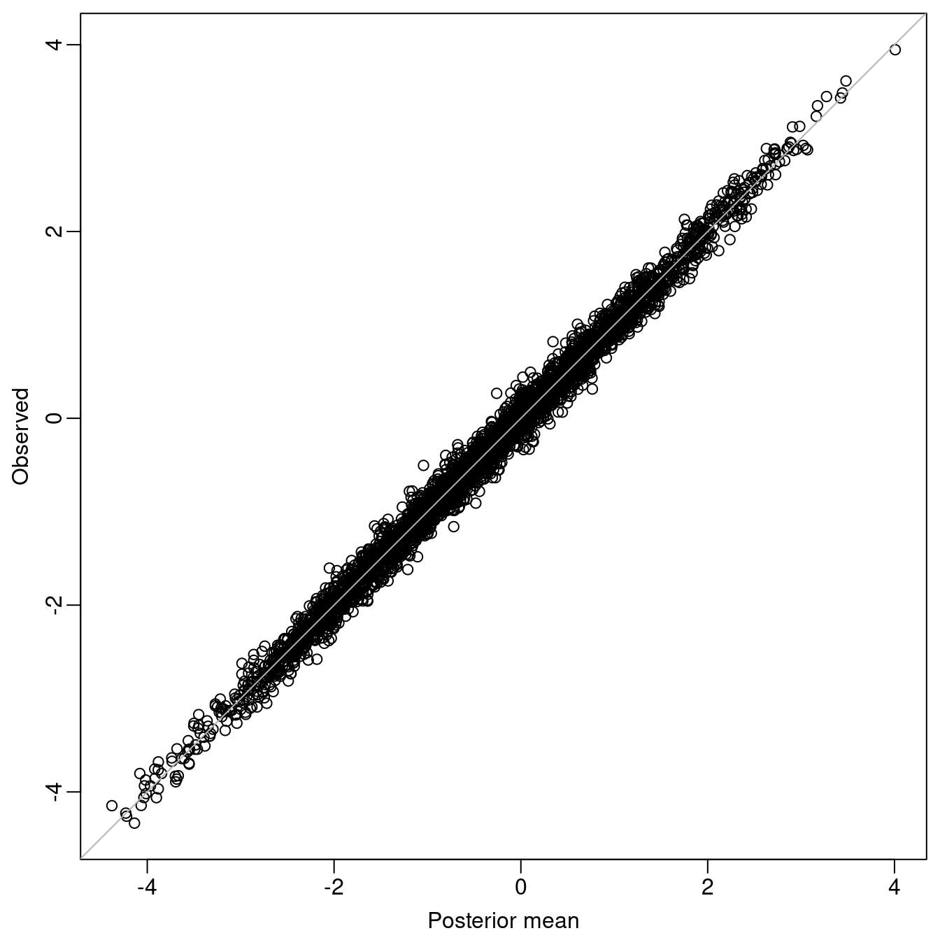
Figure 7.4: Validation: Observed values versus posterior means from the fitted model.
7.2 Continuous time domain
We now eliminate the assumption that the observations have been collected over discrete time points. This is the case for, e.g., fishing data, and space-time point processes in general. Similarly to how we use the Finite Element Method approach for space, we use a set of time knots to set up piecewise linear basis functions over time.
7.2.1 Data simulation
First, we set the spatial locations and sample time points from a continuous interval:
loc <- unique(as.matrix(PRprec[, 1:2]))
n <- nrow(loc)
time <- sort(runif(n, 0, 1))
To sample from the current model, we define a space-time separable covariance function. We use a Matérn covariance in space and exponential decaying covariance function over time:
local.stcov <- function(coords, time, kappa.s, kappa.t,
  variance = 1, nu = 1) {
  s <- as.matrix(dist(coords))
  t <- as.matrix(dist(time))
  scorr <- exp((1 - nu) * log(2) + nu * log(s * kappa.s) -
    lgamma(nu)) * besselK(s * kappa.s, nu)
  diag(scorr) <- 1
  return(variance * scorr * exp(-t * kappa.t))
}
Function local.stcov() will be used to compute the covariance function at
the simulated space-time points and to sample from the model:
kappa.s <- 1
kappa.t <- 5
s2 <- 1 / 2
xx <- crossprod(
  chol(local.stcov(loc, time, kappa.s, kappa.t, s2)),
  rnorm(n))

beta0 <- -3
tau.error <- 3

y <- beta0 + xx + rnorm(n, 0, sqrt(1 / tau.error))
7.2.2 Data stack preparation
To fit the space-time continuous model we must first define the time knots and the temporal mesh. For this, we define a one-dimensional mesh with 10 knots:
k <- 10
mesh.t <- inla.mesh.1d(seq(0 + 0.5 / k, 1 - 0.5 / k, length = k))
The knots in the resulting temporal mesh are the following:
mesh.t$loc
##  [1] 0.05 0.15 0.25 0.35 0.45 0.55 0.65 0.75 0.85 0.95
We continue using the low resolution mesh for the border of Paraná state created in Section 2.6. This means that we can also re-use the SPDE model defined in the previous example.
The index set for the spatio-temporal model can be defined as:
iset <- inla.spde.make.index('i', n.spde = spde$n.spde,
  n.group = k)
The projection matrix considers both the spatial and temporal projection.
Hence, it needs
the spatial mesh and the spatial locations,
the time points and the temporal mesh.
These are passed to function inla.spde.make.A as follows:
A <- inla.spde.make.A(mesh = prmesh1, loc = loc,
  group = time, group.mesh = mesh.t)
The effects in the data stack are a list with two elements:
the index set for the spatial effect and the categorical covariate.
The stack data is defined as:
sdat <- inla.stack(
  data = list(y = y),
  A = list(A,1),
  effects = list(iset, list(b0 = rep(1, n))),
  tag = "stdata")
7.2.3 Fitting the model and some results
An exponential correlation function is used for time with parameter \(\kappa\) as the inverse range parameter. It gives a correlation between time knots equal to:
exp(-kappa.t * diff(mesh.t$loc[1:2]))
## [1] 0.6065
We fit the model using an AR(\(1\)) temporal correlation over the time knots as follows:
formulae <- y ~ 0 + b0 + f(i, model = spde, group = i.group,
  control.group = list(model = 'ar1', hyper = h.spec))

res <- inla(formulae, data = inla.stack.data(sdat),
  control.family = list(hyper = list(prec = prec.prior)),
  control.predictor = list(compute = TRUE,
    A = inla.stack.A(sdat)))
We summarize the posterior marginal distributions for the likelihood precision and the random field parameters:
res$summary.hyperpar
##                                           mean      sd
## Precision for the Gaussian observations 2.6548 0.17703
## Range for i                             2.9089 0.72622
## Stdev for i                             0.6453 0.07635
## GroupRho for i                          0.3056 0.21392
##                                         0.025quant 0.5quant
## Precision for the Gaussian observations     2.3213   2.6498
## Range for i                                 1.7559   2.8158
## Stdev for i                                 0.5090   0.6405
## GroupRho for i                             -0.1572   0.3241
##                                         0.975quant   mode
## Precision for the Gaussian observations     3.0182 2.6411
## Range for i                                 4.5854 2.6382
## Stdev for i                                 0.8088 0.6310
## GroupRho for i                              0.6694 0.3707
The posterior marginal distributions of these parameters are shown in Figure 7.5, which includes the marginal distribution for the intercept, error precision, spatial range, standard deviation and temporal correlation in the space-time field.
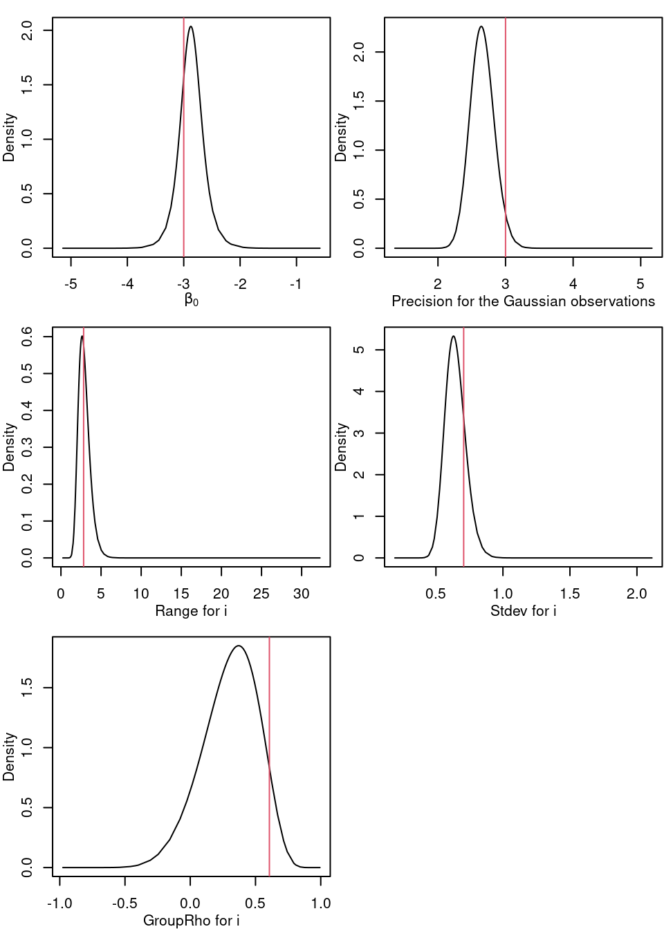
Figure 7.5: Marginal posterior distribution for the intercept, likelihood precision and the parameters in the space-time process.
7.3 Lowering the resolution of a spatio-temporal model
Model fitting can be challenging when dealing with large data sets. In this section we show techniques for lowering the resolution of the representation of the space-time random effect, to make model fitting faster.
First, we build the spatial mesh and the SPDE model using the rainfall data in Paraná state with the following code:
data(PRprec)
bound <- inla.nonconvex.hull(as.matrix(PRprec[, 1:2]), 0.2, 0.2,
  resol = 50)
mesh.s <- inla.mesh.2d(bound = bound, max.edge = c(1,2),
  offset = c(1e-5, 0.7), cutoff = 0.5)
spde.s <- inla.spde2.matern(mesh.s)
7.3.1 Data temporal aggregation
In this subsection we set up the data that we will use for the example in the next subsection.
The reader may consider the dataframe df as an original binomial dataset, and how it was constructed is not of any large importance.
The data we analyze are composed of 616 location points observed over 365 days
in Paraná state (Brazil). The response variable is daily rainfall. The
dimension of the data.frame with this dataset and the first 7 variables
from the first two rows:
dim(PRprec)
## [1] 616 368
PRprec[2:3, 1:7]
##   Longitude Latitude Altitude d0101 d0102 d0103 d0104
## 3    -50.77   -22.96      344     0     1     0   0.0
## 4    -50.65   -22.95      904     0     0     0   3.3
In this example the aim is to analyze the probability of rain. Therefore we now convert this continuous dataset of rainfall amount into occurrence of rain. The response variable is whether rainfall was higher than \(0.1\) or not.
PRoccurrence = 0 + (PRprec[, -c(1, 2, 3)] > 0.1)
PRoccurrence[2:3, 1:7]
##   d0101 d0102 d0103 d0104 d0105 d0106 d0107
## 3     0     1     0     0     0     0     1
## 4     0     0     0     1     0     0     1
To reduce the size of the dataset, we will aggregate by summing over five consecutive days. We would model the original dataset with a Bernoulli, therefore the aggregated dataset is modeled by a binomial (because a sum of Bernoulli variables is binomial distributed). There will be many 5 day blocks with less than 5 observations, because of missing values, and these will give binomials with less than 5 trials.
First, a new index is created to group the days in groups of five days:
id5 = rep(1:(365 / 5), each = 5)The number of raining days is obtained with:
y5 <- t(apply(PRoccurrence[, 1:365], 1, tapply, id5, sum,
  na.rm = TRUE))
table(y5)
## y5
##     0     1     2     3     4     5
## 17227 10608  7972  4539  3063  1559
Next, the number of days with observed data in each group of 5 days, i.e. the trials in our binomial likelihood, is computed as:
n5 <- t(apply(!is.na(PRprec[, 3 + 1:365]), 1, tapply, id5, sum))
table(as.vector(n5))
##
##     0     1     2     3     4     5
##  3563    77    72    95   172 40989
Now, the aggregated data has 73 time points.
From the table above, it can be seen how there are 3563 periods of
five days with no data recorded. The first approach when dealing with these
missing values could be to remove such pairs of data, both \(y\) and \(n\). If
these are not removed, value NA has to be assigned to \(y\) when \(n=0\).
However, \(n\) needs to be assigned a positive value (e.g., five).
This is done as follows:
y5[n5 == 0] <- NA
n5[n5 == 0] <- 5
We set up all the variables in a dataframe:
n <- nrow(PRprec)
df = data.frame(y = as.vector(y5), ntrials = as.vector(n5),
  locx = rep(PRprec[, 1], k),
  locy = rep(PRprec[, 2], k),
  time = rep(1:k, each = n),
  station.id = rep(1:n, k))

summary(df)
##        y           ntrials          locx            locy
##  Min.   :0      Min.   :1.00   Min.   :-54.5   Min.   :-26.9
##  1st Qu.:0      1st Qu.:5.00   1st Qu.:-52.9   1st Qu.:-25.6
##  Median :1      Median :5.00   Median :-51.7   Median :-24.9
##  Mean   :1      Mean   :4.98   Mean   :-51.6   Mean   :-24.7
##  3rd Qu.:2      3rd Qu.:5.00   3rd Qu.:-50.4   3rd Qu.:-23.8
##  Max.   :5      Max.   :5.00   Max.   :-48.2   Max.   :-22.5
##  NA's   :3563
##       time      station.id
##  Min.   : 1   Min.   :  1
##  1st Qu.:19   1st Qu.:155
##  Median :37   Median :308
##  Mean   :37   Mean   :308
##  3rd Qu.:55   3rd Qu.:462
##  Max.   :73   Max.   :616
##
7.3.2 Reducing the temporal resolution
This approach can be seen in the template code in Section 3.2 in Lindgren and Rue (2015) and has also been considered in the last example in Blangiardo and Cameletti (2015). The main idea is to place some knots over the time window and define the model at such knots. Then, the projection is defined from the time knots, similarly as is done for the spatial case with the mesh.
The knots are placed at every 6 time points of the temporally aggregated data, which has 73 time points altogether. So, in the end there are only 12 knots over time.
bt <- 6
gtime <- seq(1 + bt, k, length = round(k / bt)) - bt / 2
mesh.t <- inla.mesh.1d(gtime, degree = 1)
The model dimension is then 1152.
Then, when the projection matrix is computed, it is necessary to consider the temporal mesh and the group index in the scale of the data to be analyzed. The projection matrix with the definition of the spatial and temporal meshes used above can be obtained as follows:
Ast <- inla.spde.make.A(mesh = mesh.s,
 loc = cbind(df$locx, df$locy), group.mesh = mesh.t,
 group = df$time)
The index set and the data stack are built as usual:
idx.st <- inla.spde.make.index('i', n.spde = spde.s$n.spde,
  n.group = mesh.t$n)
stk <- inla.stack(
  data = list(y = df$y, ntrials = df$ntrials),
  A = list(Ast, 1),
  effects = list(idx.st, data.frame(mu0 = 1,
    altitude = rep(PRprec$Altitude / 1000, k))))
Note that in the previous code the values of the altitude have been rescaled by dividing them by 1000. In general, we need to rescale the covariates to get stable numerical inference.
The formula is also the usual for a separable spatio-temporal model:
form <- y ~ 0 + mu0 + altitude + f(i, model = spde.s,
  group = i.group, control.group = list(model = 'ar1',
    hyper = list(rho = list(prior = 'pc.cor1', param = c(0.7, 0.7)))))
In order to reduce computational time in this example, a number of options will
be set in the call to inla(). In particular, the adaptive
approximation (strategy = 'adaptive') and the Empirical Bayes integration
strategy over the hyperparameters (int.strategy = 'eb') will be used. These
options are passed in the control.inla argument of inla(). Furthermore,
we start the optimizer at the initial values init:
# Initial values of hyperparameters
init = c(-0.5, -0.9, 2.6)
# Model fitting
result <- inla(form, 'binomial', data = inla.stack.data(stk),
  Ntrials = inla.stack.data(stk)$ntrials,
  control.predictor = list(A = inla.stack.A(stk), link = 1),
  control.mode = list(theta = init, restart = TRUE),
  control.inla = list(strategy = 'adaptive', int.strategy = 'eb'))
The fitted spatial effect can be plotted for each temporal knot and overlay the proportion of raining days considering the data closest to the time knots. First, a grid to make the projection is required:
data(PRborder)
r0 <- diff(range(PRborder[, 1])) / diff(range(PRborder[, 2]))
prj <- inla.mesh.projector(mesh.s, xlim = range(PRborder[, 1]),
  ylim = range(PRborder[, 2]), dims = c(100 * r0, 100))
in.pr <- inout(prj$lattice$loc, PRborder)
Next, the projection of the posterior mean fitted at each time knot is computed:
mu.st <- lapply(1:mesh.t$n, function(j) {
  idx <- 1:spde.s$n.spde + (j - 1) * spde.s$n.spde
  r <- inla.mesh.project(prj,
    field = result$summary.ran$i$mean[idx])
  r[!in.pr] <- NA
  return(r)
})
These projections are shown in Figure 7.6. We add the locations points with point size proportional to the rain occurrence in each period.
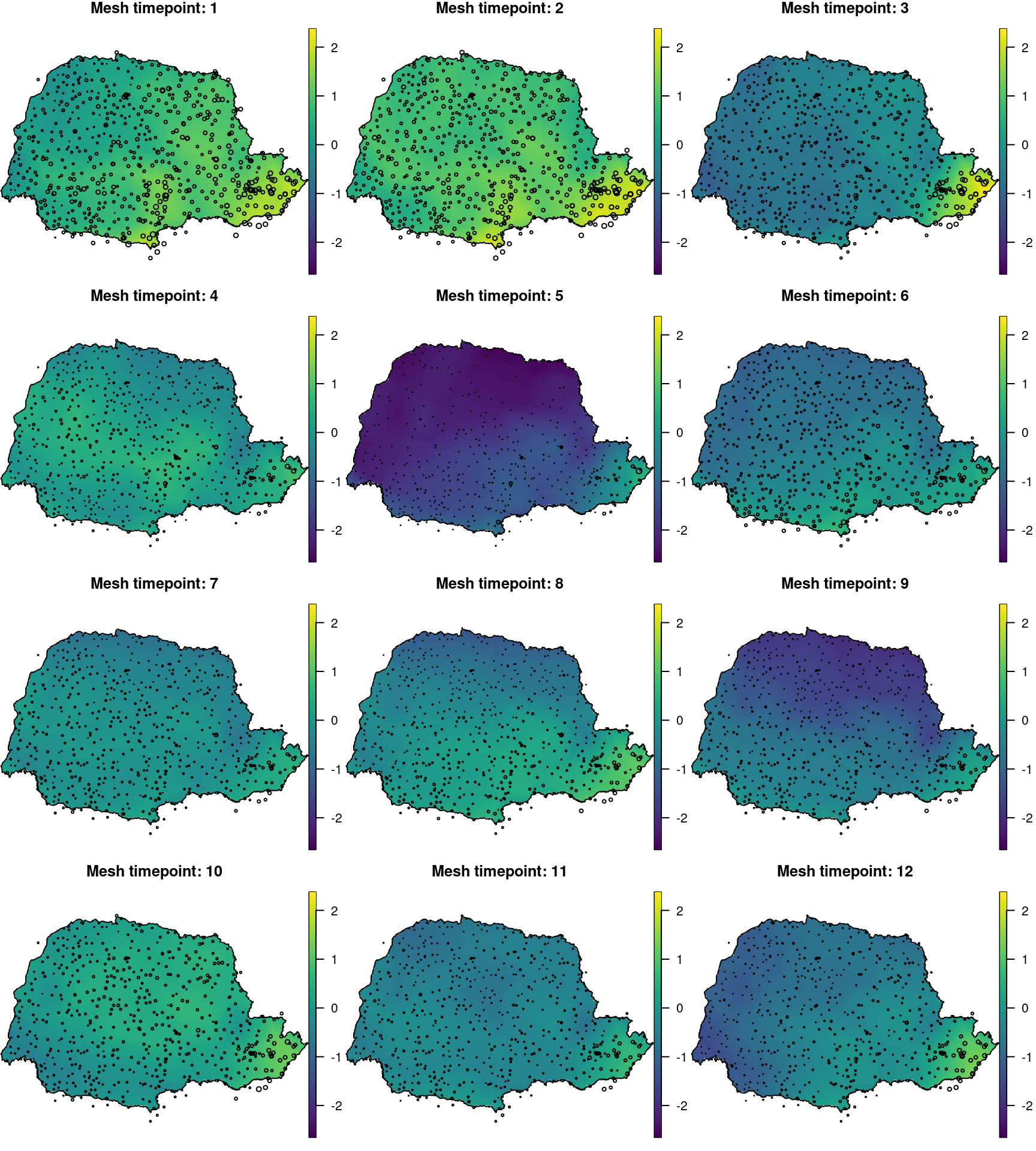
Figure 7.6: Spatial effect at each time knot obtanined with the spatio-temporal model fitted to the number of raining days in Paraná state (Brazil).
7.4 Conditional simulation: Combining two meshes
7.4.1 Motivation
There are a number of prediction problems that require modeling and prediction of the spatial, or spatio-temporal phenomenon over an extensive region, such as a country. However, in many situations, observations are only available in a limited part of the region. In this section we will discuss how to deal with this in a computationally efficient manner. Although practical computational issues are more common when dealing with spatio-temporal data, the example developed here focuses on spatial data to simplify the presentation. The same principle can be, however, easily extended to the spatio-temporal case.
We illustrate the case where there is a process that is only observed in part of the study region by using locations from Paraná state in Brazil. We use the boundary domain of the Paraná state and assume that we only have data from the left half part of the Paraná, while spatial prediction is desired for the entire state. Additionally, we consider fitting the model using a mesh around the available data and predicting using a mesh over the entire area of interest. These has been obtained with the following code and the resulting dataset has been plotted in Figure 7.7.
# loading the Parana border and precipitation data
data(PRborder)
data(PRprec)

# Which data points fall inside the left 50% of Parana
mid.long <- mean(range(PRborder[, 1]))
sel.loc <- which(PRprec[, 1] < mid.long)
sel.bor <- which(PRborder[, 1] < mid.long)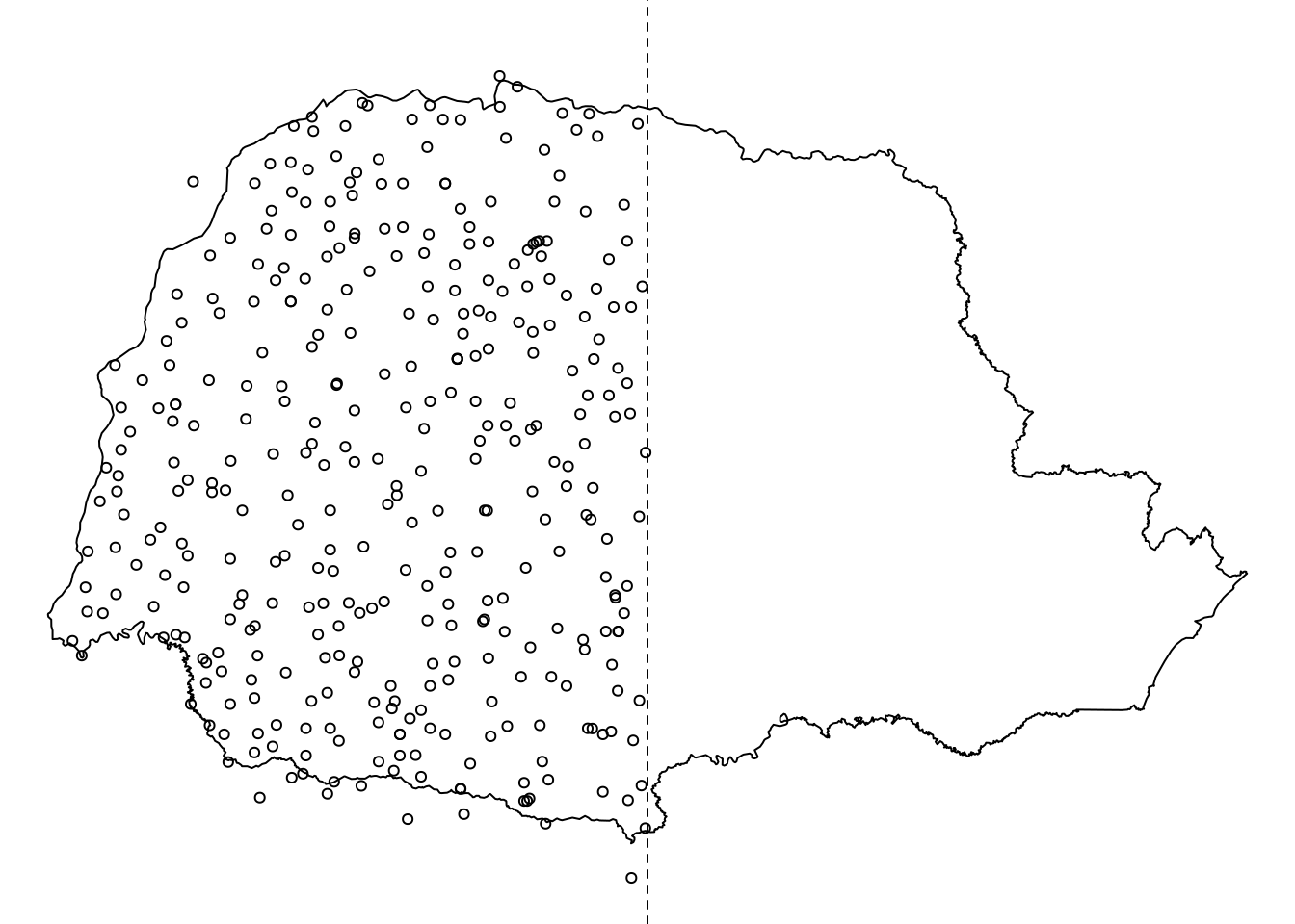
Figure 7.7: Problem setting: available data over half of the domain.
One way to obtain such predictions is to fit the model using a mesh that
contains both, the locations where data is observed and the prediction
locations (denoted by mesh2). Here we show a more efficient way, where the
model is fitted using a mesh only around where the observations are placed
(denoted by mesh1), and then conditional simulations are used to predict at
the nodes of mesh2. This is achieved by taking advantage of numerical
methods for sparse matrices applied to conditional simulation of GRMFs and the
result is a considerable speedup in the computations when comparing to fitting
the model directly using mesh2. After conditioning, the predictions at the
data locations will be exactly the same values obtained from the fit using
mesh1. In the geostatistics literature, this can be achieved with
conditioning by kriging. The basis of the conditioning approach is to use the
same covariance function for both the unconditional simulations and the
predictions.
This is equivalent to the problem of sampling from a GMRF under the linear constraint
\[\begin{align} \mathbf{Ax} = \mathbf{b}, \end{align}\]
where \(\mathbf{A}\) is a \(n_1 \times n_2\) matrix, with \(n_1\) and \(n_2\) being the number of nodes in mesh1 and mesh2, respectively.
The vector \(\mathbf{b}\) is the vector of constraints of length \(n_1\) and corresponds to the predicted latent field from the fit using mesh1.
A way to obtain the correct conditional distribution of \(\mathbf{x}^{*}\) is to sample from the unconstrained GMRF \(\mathbf{x} \sim \textrm{N}(\boldmath{\mu}, \mathbf{Q}^{-1})\) and then compute
\[\begin{align} \tag{7.1} \mathbf{x}^{*} = \mathbf{x} - \mathbf{Q}^{-1}\mathbf{A}^{T}(\mathbf{AQ}^{-1}\mathbf{A}^{T})^{-1}(\mathbf{Ax}-\mathbf{b}), \end{align}\]
where \(\mathbf{Q}\) is a \(n_2 \times n_2\) precision matrix and \(\mathbf{AQ}^{-1}\mathbf{A}^{T}\) is a dense matrix with dimensions equal to the number of constrains, that is, \(n_1 \times n_1\). To factorize \(\mathbf{AQ}^{-1}\mathbf{A}^{T}\), we can take advantage of the sparse structure of \(\mathbf{Q}\) and obtain fast computations for \(n_1 \ll n_2\).
7.4.2 Paraná state example
At each location \(i\), we suppose the following distribution for the data \(y_i\):
\[\begin{align} y_i \sim \textrm{N}(\eta_i, \sigma_{\epsilon}), \end{align}\]
with \(\sigma_{\epsilon}\) being an iid Gaussian noise and \(\eta_i\) being the linear predictor, defined as:
\[\begin{align} \eta_i = \beta_0 + u_i, \end{align}\]
where \(\beta_0\) is the intercept and \(u_i\) is a realization of a spatial random Gaussian field with Matérn covariance at the data locations \(i\).
We use simulated data to show how to obtain predictions in mesh2 after
fitting the model using mesh1. To illustrate the ability of our method to
predict using a different mesh, we assume that the data comes from the random
field based on mesh2, namely \(u_i\).
We build mesh1 considering only the data from the western half of Paraná
state:
#  Building mesh1
mesh1 <- inla.mesh.2d(loc = PRprec[sel.loc, 1:2], max.edge = 1,
  cutoff = 0.1, offset = 1.2)
Next, we create mesh2 such that all the nodes from mesh1 are also nodes of mesh2.
In addition, we use the border of the Paraná state to define the high resolution interior of the mesh2.
In order to implement both these restrictions we first create an auxiliary mesh mesh2a considering the border of the Paraná state.
Then we use the locations from mesh1 and from the auxiliary mesh to create mesh2.
# define a boundary for the Parana border and an auxiliary mesh
ibound <- inla.nonconvex.hull(PRborder, 0.05, 2, resol = 250)
mesh2a <- inla.mesh.2d(mesh1$loc, boundary = ibound,
  max.edge = 0.2, cutoff = 0.1)
# Building mesh2 considering wider a boundary
bound <- inla.nonconvex.hull(PRborder, 2)
mesh2 <- inla.mesh.2d(loc = rbind(mesh1$loc, mesh2a$loc),
  boundary = bound, max.edge = 1, cutoff = 0.1)
As a result, mesh1 has 381 nodes and mesh2 has 1469 nodes.
We can see these two meshes in Figure 7.8.
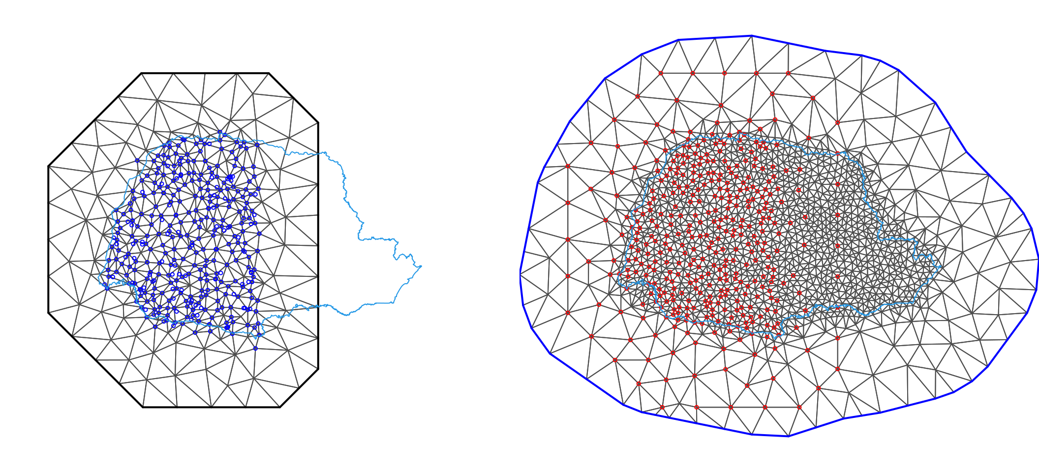
Figure 7.8: The first mesh, together with the data locations in blue (left). Mesh mesh2, which will be used for predictions, and the points of the first mesh represented as red points (right). The inner blue polygon shows the Paraná state border.
To simulate data, we need to fix the range and standard deviation and then define the SPDE models for both meshs as follows:
# SPDE model parameters
range <- 3
std.u <- 1
# Define the SPDE models for mesh1 and mesh2
spde1 = inla.spde2.pcmatern(mesh1, prior.range = c(1, 0.1),
  prior.sigma = c(1, 0.1))
spde2 = inla.spde2.pcmatern(mesh2, prior.range = c(1, 0.1),
  prior.sigma = c(1, 0.1))
The precision matrices for both SPDE models are built with:
# Obtain the precision matrix for spde1 and spde2
Q1 = inla.spde2.precision(spde1,
  theta = c(log(range), log(std.u)))
Q2 = inla.spde2.precision(spde2,
  theta = c(log(range), log(std.u)))
Simulation of the random field at the nodes of mesh2 can be performed as follows:
u <- as.vector(inla.qsample(n = 1, Q = Q2, seed = 1))We complete the data simulation by projecting the mesh nodes into the observed
data points and adding an iid noise. We also build the projection matrix for
mesh1, which will be used for fitting the model:
A1 <- inla.spde.make.A(mesh1,
  loc = as.matrix(PRprec[sel.loc, 1:2]))
A2 <- inla.spde.make.A(mesh2,
  loc = as.matrix(PRprec[sel.loc, 1:2]))
We now sample the spatial field and iid Gaussian noise at the observation locations:
std.epsilon = 0.1
y <- drop(A2 %*% u) + rnorm(nrow(A2), sd = std.epsilon)
The stack data includes the intercept and the SPDE model defined at mesh1:
stk <- inla.stack(
  data = list(resp = y),
  A = list(A1, 1),
  effects = list(i = 1:spde1$n.spde,m = rep(1, length(y))),
  tag = 'est')
7.4.3 Fitting the model
The model is fitted as follows:
res <- inla(resp ~ 0 + m + f(i, model = spde1),
  data = inla.stack.data(stk),
  control.compute = list(config = TRUE),
  control.predictor = list(A = inla.stack.A(stk)))
The summary of the posterior marginal distribution for the standard deviation of the noise, the range and the standard deviation, together with the true values is shown below.
# Marginal for standard deviation of Gaussian likelihood
p.s.eps <- inla.tmarginal(function(x) 1 / sqrt(exp(x)),
  res$internal.marginals.hyperpar[[1]])
# Summary of post. marg. of st. dev.
s.std <- unlist(inla.zmarginal(p.s.eps, silent = TRUE))[c(1:3, 7)]

hy <- cbind(True = c(std.epsilon, range, std.u),
 rbind(s.std, res$summary.hyperpar[2:3, c(1:3, 5)]))
rownames(hy) <- c('Std epsilon', 'Range field', 'Std field')
hy
##             True   mean       sd 0.025quant 0.975quant
## Std epsilon  0.1 0.1013 0.006678    0.08895     0.1152
## Range field  3.0 3.5706 0.902238    2.30850     5.7923
## Std field    1.0 1.1046 0.254259    0.74172     1.7247
7.4.4 Obtaining predictions
Before proceeding to the actual prediction, we need to sample from the posterior distribution using the fitted model. We draw 100 samples from the posterior considering the internal parametrization for the hyperparameters with:
nn <- 100
s <- inla.posterior.sample(n = nn, res, intern = TRUE,
  seed = 1, add.names = FALSE)
We can find the indices for the spatial random effect \(i\) in the following way:
## Find the values of latent field "i" in samples from mesh1
contents <- res$misc$configs$contents
effect <- "i"
id.effect <- which(contents$tag == effect)
ind.effect <- contents$start[id.effect] - 1 +
  (1:contents$length[id.effect])
For each sample from the posterior distribution, the following code produces
predictions of the latent field \(\mathbf{u}\) at the nodes of mesh2
constrained on the predictions at the nodes of mesh1 being equal of the
values of the latent field from the posterior samples generated from fitting
the model with mesh1. This code is based on Equation (7.1), but
with additional complications to achieve greater computational speed:
# Obtain predictions at the nodes of mesh2
loc1 = mesh1$loc[,1:2]
loc2 = mesh2$loc[,1:2]
n = mesh2$n

mtch = match(data.frame(t(loc2)), data.frame(t(loc1)))
idx.c = which(!is.na(mtch))
idx.u = setdiff(1:mesh2$n, idx.c)
p = c(idx.u, idx.c)

ypred.mesh2 = matrix(c(NA), mesh2$n, nn)

m <- n - length(idx.c)
iperm <- numeric(m)

t0 <- Sys.time()
for(ind in 1:nn){

  Q.tmp = inla.spde2.precision(spde2,
    theta = s[[ind]]$hyperpar[2:3])

  Q = Q.tmp[p, p]
  Q.AA = Q[1:m, 1:m]
  Q.BB = Q[(m + 1):n, (m + 1):n]
  Q.AB = t(Q[(m + 1):n, 1:m])
  Q.AA.sf = Cholesky(Q.AA,  perm = TRUE,  LDL = FALSE)
  perm = Q.AA.sf@perm + 1
  iperm[perm] = 1:m
  x = solve(Q.AA.sf, rnorm(m), system = "Lt")
  xc = s[[ind]]$latent[ind.effect]
  xx = solve(Q.AA.sf, -Q.AB %*% xc,  system = "A")

  x = rep(NA, n)
  x[idx.u] = c(as.matrix(xx))
  x[idx.c] = xc

  ypred.mesh2[, ind] = x
}
Sys.time() - t0
## Time difference of 1.928 secs
Notice that the code above computes the Cholesky factorization of the precision matrix \(\mathbf{Q}\) rapidly by taking the sparsity of this matrix into account.
This makes it possible to obtain fast predictions in a large number of locations.
Another possibility is to fit the model directly using mesh2 instead of mesh1.
However, this would require a lot more computational time and results would be similar to the procedure shown here.
To produce maps of the predicted random field in a fine grid, we compute a projection matrix for a grid of points over a square that contains the locations of the border of the Paraná state.
# Projection from the mesh nodes to a fine grid
projgrid  <- inla.mesh.projector(mesh2,
  xlim = range(PRborder[, 1]), ylim = range(PRborder[, 2]),
  dims = c(300, 300))
Then, we can obtain the projection of the simulated random field and compare with the projection of the posterior mean of the predictions. Missing values are assigned to the grid points that are outside of the Paraná state:
# Find points inside the state of Parana
xy.in <- inout(projgrid$lattice$loc, PRborder[, 1:2])
# True field
r1 <- inla.mesh.project(projgrid , field = u)
r1[!xy.in] <- NA

# Mean predicted random field
r2 <- inla.mesh.project(projgrid , field = rowMeans(ypred.mesh2))
r2[!xy.in] <- NA

# sd of the predicted random field
sd.r2 <- inla.mesh.project(
  projgrid, field=apply(ypred.mesh2, 1, sd, na.rm = TRUE))
sd.r2[!xy.in] <- NA

# plotting
par(mfrow = c(3, 1), mar = c(0, 0, 0, 0))
zlm <- range(c(r1, r2), na.rm = TRUE)

# Map of the true field
book.plot.field(list(x = projgrid$x, y = projgrid$y, z = r1),
  zlim = zlm)
points(PRprec[sel.loc, 1:2], col = "black", asp = 1, cex = 0.3)

## Map of the mean of the mean predicted random field
book.plot.field(list(x = projgrid$x, y = projgrid$y, z = r2),
  zlim = zlm)
points(PRprec[sel.loc, 1:2], col = "black", asp = 1, cex = 0.3)

book.plot.field(list(x = projgrid$x, y = projgrid$y, z = sd.r2))
points(PRprec[sel.loc, 1:2], col = "black", asp = 1, cex = 0.3)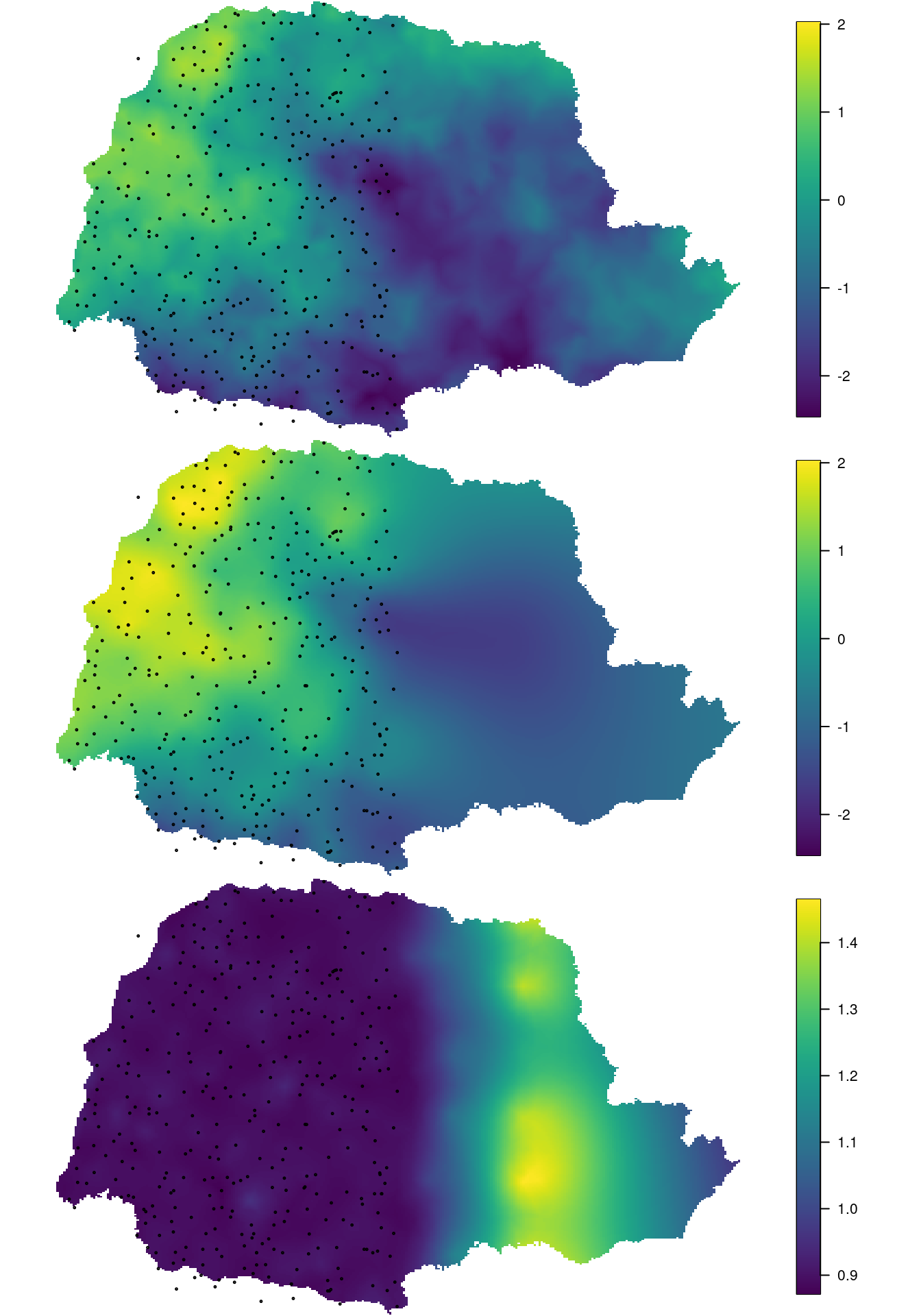
Figure 7.9: The simulated field (top), the estimated posterior mean (middle) and the posterior marginal standard deviation (bottom).
References
Blangiardo, M., and M. Cameletti. 2015. Spatial and SpatioTemporal Bayesian Models with R-INLA. Chichester, UK: John Wiley & Sons, Ltd.
Cameletti, M., F. Lindgren, D. Simpson, and H. Rue. 2013. “Spatio-Temporal Modeling of Particulate Matter Concentration Through the Spde Approach.” Advances in Statistical Analysis 97 (2): 109–31.
Fuglstad, G-A., D. Simpson, F. Lindgren, and H. Rue. 2018. “Constructing Priors That Penalize the Complexity of Gaussian Random Fields.” Journal of the American Statistical Association to appear. https://doi.org/10.1080/01621459.2017.1415907.
Lindgren, F., and H. Rue. 2015. “Bayesian Spatial and Spatio-Temporal Modelling with R-INLA.” Journal of Statistical Software 63 (19).
Rue, H., and L. Held. 2005. Gaussian Markov Random Fields: Theory and Applications. Monographs on Statistics & Applied Probability. Boca Raton, FL: Chapman & Hall.