Chapter 3 More than one likelihood

Chapters 1 and 2 have focused on describing the INLA and SPDE methodologies, respectively. In this chapter we introduce more complex models that require the use of several likelihoods. These examples will focus on models with a multivariate response, how to deal with measurement error and using part of the linear predictor of one variable as part of the linear predictor of another variable.

3.1 Coregionalization model

3.1.1 Motivation

In this section we present a way to fit the Bayesian coregionalization model similar to the ones proposed by Schmidt and Gelfand (2003) and Gelfand, Schmidt, and Sirmans (2002). A related code example to the one we present here can be found in Chapter 8 in Blangiardo and Cameletti (2015). These models are often used when measurement stations record several variables; for example, a station measuring pollution may register values of CO2, CO and NO2. Instead of modeling these as several univariate datasets, the models we present in this section deal with the joint dependency structure. Dependencies among the different outcomes are modeled through shared components at the predictor level.

Usually, in coregionalization models, the different responses are assumed to be observed at the same locations. With the INLA-SPDE approach, we do not require the different outcome variables to be measured at the same locations. Hence, in the code example below we show how to model responses observed at different locations. In this section we present a spatial model, and in Section 8.1 we generalize it to the space-time setting.

3.1.2 The model and parametrization

The case of three outcomes is defined considering the following equations:

\[\begin{align*} y_1(\mathbf{s}) &= \alpha_1 + z_1(\mathbf{s}) + e_1(\mathbf{s}) \\ y_2(\mathbf{s}) &= \alpha_2 + \lambda_1 z_1(\mathbf{s}) + z_2(\mathbf{s}) + e_2(\mathbf{s}) \\ y_3(\mathbf{s}) &= \alpha_3 + \lambda_2 z_1(\mathbf{s}) + \lambda_3 z_2(\mathbf{s}) + z_3(\mathbf{s}) + e_3(\mathbf{s}), \end{align*}\]

where the \(\alpha_k\) are intercepts, \(z_{k}(\mathbf{s})\) are spatial effects, \(\lambda_k\) are weights for some of the spatial effects and \(e_{k}(\mathbf{s})\) are uncorrelated error terms, with \(k=1,2,3\).

This model can be fitted with INLA using the copy feature, which is explained in more detail in Section 1.6.2 and Section 3.3. In INLA, there is only one single linear predictor (one single formula). Thus, to implement the above three equations, we have to stack the linear predictors together into one long vector. Because of this, we have to copy the spatial effects \(z_1(\mathbf{s})\) and \(z_2(\mathbf{s})\) to represent the different contributions to the different parts of the formula.

3.1.3 Data simulation

The following parameters are used to simulate data from the model presented above:

# Intercept on reparametrized model
alpha <- c(-5, 3, 10) 
# Random field marginal variances
m.var <- c(0.5, 0.4, 0.3) 
# GRF range parameters:
range <- c(4, 3, 2)
# Copy parameters: reparameterization of coregionalization 
# parameters
beta <- c(0.7, 0.5, -0.5) 
# Standard deviations of error terms
e.sd <- c(0.3, 0.2, 0.15)

Similarly, the number of observations of each response variable is defined as follows:

n1 <- 99
n2 <- 100
n3 <- 101

In this example, we use a different number of observations for each response variable, and they are observed at different locations. In typical applications of coregionalization, however, all response variables will be measured at the same locations The location points are sampled at random on a \((0,10)\times(0,5)\) rectangular domain.

loc1 <- cbind(runif(n1) * 10, runif(n1) * 5) 
loc2 <- cbind(runif(n2) * 10, runif(n2) * 5) 
loc3 <- cbind(runif(n3) * 10, runif(n3) * 5) 

The book.rMatern() function described in Section 2.1.3 will be used to simulate independent random field realizations for each time. The three random fields are simulated as follows. Note that we need, for example, the locations loc2 for the field u1 because this field is also used for the second variable.

set.seed(05101980)
z1 <- book.rMatern(1, rbind(loc1, loc2, loc3), range = range[1],
  sigma = sqrt(m.var[1]))
z2 <- book.rMatern(1, rbind(loc2, loc3), range = range[2],
  sigma = sqrt(m.var[2]))
z3 <- book.rMatern(1, loc3, range = range[3],
  sigma = sqrt(m.var[3]))

Finally, we obtain samples from the observations:

set.seed(08011952)

y1 <- alpha[1] + z1[1:n1] + rnorm(n1, 0, e.sd[1])
y2 <- alpha[2] + beta[1] * z1[n1 + 1:n2] + z2[1:n2] + 
  rnorm(n2, 0, e.sd[2])
y3 <- alpha[3] + beta[2] * z1[n1 + n2 + 1:n3] + 
  beta[3] * z2[n2 + 1:n3] + z3 + rnorm(n3, 0, e.sd[3])

3.1.4 Model fitting

This model only requires one mesh to fit all of the three spatial random fields. This makes it easier to link the different effects across different outcomes at different spatial locations. We choose to use all the locations when creating the mesh, as follows:

mesh <- inla.mesh.2d(rbind(loc1, loc2, loc3), 
  max.edge = c(0.5, 1.25), offset = c(0.1, 1.5), cutoff = 0.1)

The next step is defining the SPDE model considering the PC-prior derived in Fuglstad et al. (2018) and described in Sections 1.6.5 and 2.3:

spde <- inla.spde2.pcmatern(
  mesh = mesh,
  prior.range = c(0.5, 0.01), # P(range < 0.5) = 0.01
  prior.sigma = c(1, 0.01)) # P(sigma > 1) = 0.01

For each of the parameters (i.e., coefficients) of the copied effects, the prior is Gaussian with zero mean and precision 10. These are defined as follows:

hyper <- list(beta = list(prior = 'normal', param = c(0, 10)))

The formula including all the terms in the model is defined as follows:

form <- y ~ 0 + intercept1 + intercept2 + intercept3 + 
  f(s1, model = spde) + f(s2, model = spde) + 
  f(s3, model = spde) + 
  f(s12, copy = "s1", fixed = FALSE, hyper = hyper) + 
  f(s13, copy = "s1", fixed = FALSE, hyper = hyper) + 
  f(s23, copy = "s2", fixed = FALSE, hyper = hyper) 

Similarly, the projection matrices for each set of locations are obtained as:

A1 <- inla.spde.make.A(mesh, loc1) 
A2 <- inla.spde.make.A(mesh, loc2) 
A3 <- inla.spde.make.A(mesh, loc3) 

We organize the data by defining three stacks and then joining them:

stack1 <- inla.stack(
  data = list(y = cbind(as.vector(y1), NA, NA)),
  A = list(A1), 
  effects = list(list(intercept1 = 1, s1 = 1:spde$n.spde))) 

stack2 <- inla.stack(
  data = list(y = cbind(NA, as.vector(y2), NA)),
  A = list(A2), 
  effects = list(list(intercept2 = 1, s2 = 1:spde$n.spde, 
    s12 = 1:spde$n.spde)))

stack3 <- inla.stack(
  data = list(y = cbind(NA, NA, as.vector(y3))),
  A = list(A3), 
  effects = list(list(intercept3 = 1, s3 = 1:spde$n.spde, 
    s13 = 1:spde$n.spde, s23 = 1:spde$n.spde)))

stack <- inla.stack(stack1, stack2, stack3) 

We use a PC prior for the error precision (see Section 1.6.5):

hyper.eps <- list(hyper = list(prec = list(prior = 'pc.prec', 
  param = c(1, 0.01))))

In this model there are 12 hyperparameters in total; two hyperparameters for each of the three spatial effects, one for each likelihood, and three copy parameters. To make the optimization process fast, the parameter values used in the simulation (plus some random noise) will be set as the initial values:

theta.ini <- c(log(1 / e.sd^2), 
  c(log(range), 
    log(sqrt(m.var)))[c(1, 4, 2, 5, 3, 6)], beta)
# We jitter the starting values to avoid artificially recovering 
# the true values
theta.ini = theta.ini + rnorm(length(theta.ini), 0, 0.1)

Given that this model is complex and may take a long time to run, the empirical Bayes approach will be used, by setting int.strategy = 'eb' below, instead of integrating over the space of hyperparameters. The model is fitted with the following R code:

result <- inla(form, rep('gaussian', 3), 
  data = inla.stack.data(stack), 
  control.family = list(hyper.eps, hyper.eps, hyper.eps), 
  control.predictor = list(A = inla.stack.A(stack)),
  control.mode = list(theta = theta.ini, restart = TRUE),
  control.inla = list(int.strategy = 'eb'))

We highlight the computational time below (measured in seconds).

##      Pre  Running     Post    Total 
##   1.3627 199.3104   0.1578 200.8309

The posterior mode of the model hyperparameters is displayed in Table 3.1, using Mode = result$mode$theta. We present this table because it shows the INLA internal representation of the model parameters.

Table 3.1: Posterior modes of some of the model parameters.

Parameter	Mode
\(\log(1/\sigma^2_1)\)	2.3300
\(\log(1/\sigma^2_2)\)	3.8062
\(\log(1/\sigma^2_3)\)	3.3134
log(Range) for \(s_1\)	1.0550
log(St. Dev.) for \(s_1\)	-0.5937
log(Range) for \(s_2\)	0.9128
log(St. Dev.) for \(s_2\)	-0.5625
log(Range) for \(s_3\)	0.6617
log(St. Dev.) for \(s_3\)	-0.8283
\(\beta_1\)	0.4662
\(\beta_2\)	0.6140
\(\beta_3\)	-0.3346

We can convert the posterior marginal distributions for the likelihood precision to standard deviation with:

p.sd <- lapply(result$internal.marginals.hyperpar[1:3],
  function(m) {
    inla.tmarginal(function(x) 1 / sqrt(exp(x)), m)
  })

The posterior marginal densities of the model hyper-parameters are summarized in Table 3.2. Estimates have been put together using the following code:

# Intercepts
tabcrp1 <- cbind(true = alpha, result$summary.fixed[, c(1:3, 5)])
# Precision of the errors
tabcrp2 <- cbind(
  true = c(e = e.sd), 
  t(sapply(p.sd, function(m) 
    unlist(inla.zmarginal(m, silent = TRUE))[c(1:3, 7)])))
colnames(tabcrp2) <- colnames(tabcrp1)
# Copy parameters 
tabcrp3 <- cbind(
  true = beta, result$summary.hyperpar[10:12, c(1:3, 5)])
# The complete table
tabcrp <- rbind(tabcrp1, tabcrp2, tabcrp3)

Table 3.2: Summary of the posterior distributions of some of the parameters in the model.

Parameter	True	Mean	St. Dev.	2.5% quant.	97.5% quant.
\(\alpha_1\)	-5.00	-4.3883	0.2180	-4.8162	-3.9608
\(\alpha_2\)	3.00	2.8381	0.2206	2.4050	3.2709
\(\alpha_3\)	10.00	10.3564	0.1892	9.9850	10.7275
\(\sigma_1\)	0.30	0.3143	0.0380	0.2462	0.3953
\(\sigma_2\)	0.20	0.1499	0.0292	0.0997	0.2139
\(\sigma_3\)	0.15	0.1864	0.0429	0.1121	0.2794
\(\lambda_1\)	0.70	0.4708	0.1923	0.0953	0.8515
\(\lambda_2\)	0.50	0.6251	0.1748	0.2865	0.9734
\(\lambda_3\)	-0.50	-0.3415	0.1730	-0.6852	-0.0047

The posterior marginals of the range and the standard deviations for each field are summarized in Table 3.3.

Table 3.3: Summary of the posterior distributions of some of the parameters of the spatial fields in the model.

Parameter	True	Mean	St. Dev.	2.5% quant.	97.5% quant.
Range for s1	4.0000	3.0331	0.8967	1.6620	5.1559
Range for s2	3.0000	2.5826	0.5504	1.6849	3.8375
Range for s3	2.0000	1.9564	0.5659	1.0506	3.2524
Stdev for s1	0.7071	0.5626	0.0954	0.3997	0.7736
Stdev for s2	0.6325	0.5841	0.0948	0.4230	0.7947
Stdev for s3	0.5477	0.4438	0.0875	0.2962	0.6387

The posterior mean of each random field can be projected to the data locations. Figure 3.1 compares the fitted values to the simulated ones and it seems that the model gives good estimates of the actual values. This figure has been produced using the following code:

par(mfrow = c(2, 3), mar = c(2.5, 2.5, 1.5, 0.5),
  mgp = c(1.5, 0.5, 0))
plot(drop(A1 %*% result$summary.random$s1$mean), z1[1:n1],
  xlab = 'Posterior mean', ylab = 'Simulated', asp = 1, 
  main = 'z1 in y1')
abline(0:1)

plot(drop(A2 %*% result$summary.random$s1$mean), z1[n1 + 1:n2],
  xlab = 'Posterior mean', ylab = 'Simulated', 
  asp = 1, main = 'z1 in y2')
abline(0:1)

plot(drop(A3 %*% result$summary.random$s1$mean), 
  z1[n1 + n2 + 1:n3],
  xlab = 'Posterior mean', ylab = 'Simulated', 
  asp = 1, main = 'z1 in y3')
abline(0:1)

plot(drop(A2 %*% result$summary.random$s2$mean), z2[1:n2],
  xlab = 'Posterior mean', ylab = 'Simulated', 
  asp = 1, main = 'z2 in y2')
abline(0:1)

plot(drop(A3 %*% result$summary.random$s2$mean), z2[n2 + 1:n3],
  xlab = 'Posterior mean', ylab = 'Simulated', 
  asp = 1, main = 'z2 in y3')
abline(0:1)

plot(drop(A3 %*% result$summary.random$s3$mean), z3[1:n3],
  xlab = 'Posterior mean', ylab = 'Simulated', 
  asp = 1, main = 'z3 in y3')
abline(0:1)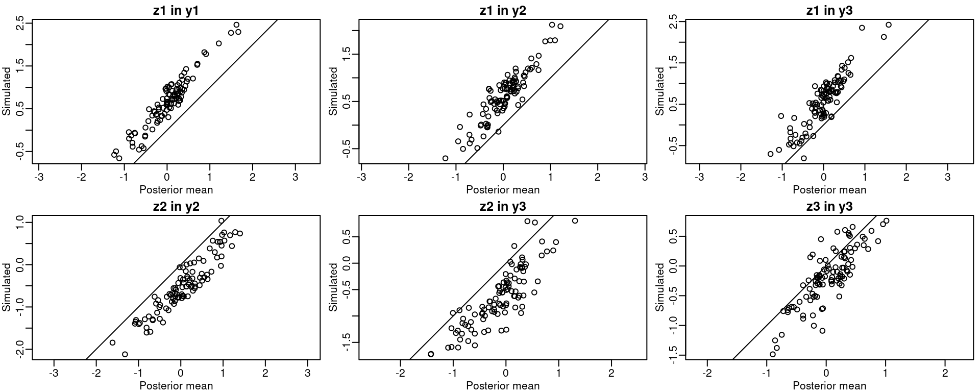

Figure 3.1: Simulated versus posterior mean fitted for the spatial fields.

3.2 Joint modeling: Measurement error model

In this section we challenge the assumption that the covariate is measured accurately. Specifically, we work with measurement error models that account for the uncertainty of covariate measurements. Introducing uncertainty in the covariate measurements is not common, not because we think covariates are perfectly measured, but because making models for measurement error is hard. In these models we have an outcome that varies over space, \(y(\mathbf{s})\), that depends on a covariate that also varies over space \(x(\mathbf{s})\). This \(x(\mathbf{s})\) is assumed to be observed with error. Further, we allow for spatial misalignment between the response \(\mathbf{y}\) and the covariate values \(\mathbf{x}\). A related example can be found in Chapter 8 of Blangiardo and Cameletti (2015).

We consider a response variable that is observed at a set of \(n_y\) locations, represented as grey dots in Figure 3.2. The covariate \(\mathbf{x}\) is observed at a set of \(n_x\) locations, shown as triangles in Figure 3.2. In some cases, \(y_i\) and \(x_i\) could be at the same location. Locations shown in Figure 3.2 are simulated by:

n.x <- 70
n.y <- 50 
set.seed(1) 
loc.y <- cbind(runif(n.y) * 10, runif(n.y) * 5) 
loc.x <- cbind(runif(n.x) * 10, runif(n.x) * 5) 

n.x <- nrow(loc.x)
n.y <- nrow(loc.y)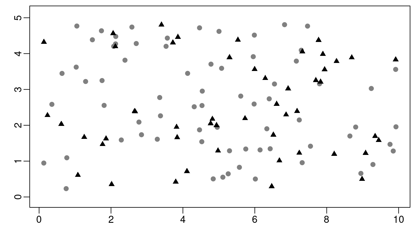 

Figure 3.2: Locations for the covariate (gray dots) and outcome (black triangles).

In this section we implement the classical measurement error (MEC, Muff et al. 2014), where we observe a proxy \(\mathbf{w}\) for \(\mathbf{x}\). Specifically, \(\mathbf{w} = \mathbf{x} + \mathbf{\epsilon}\) where the error \(\mathbf{\epsilon}\) is considered independent of \(\mathbf{x}\). Alternatively, we could assume that the error \(\mathbf{\epsilon}\) is independent of \(\mathbf{w}\); this is the so-called Berkson measurement error (Muff et al. 2014).

The linear predictor for the outcome \(\mathbf{y}\) is modeled as

\[\begin{equation} \tag{3.1} \begin{array}{rcl} \mathbf{\eta_y} & = & \alpha_y + \beta \mathbf{A}_y \mathbf{x}(\mathbf{s}) + \mathbf{A}_y\mathbf{v}(\mathbf{s}) \\ \mathbf{w} & = & \mathbf{A}_x \mathbf{x}(\mathbf{s}) + \mathbf{\epsilon} \\ \mathbf{x}(\mathbf{s}) & = & \alpha_x + \mathbf{m}(\mathbf{s}), \end{array} \end{equation}\]

where \(\alpha_y\) and \(\alpha_x\) are intercept parameters for \(\mathbf{y}\) and \(\mathbf{x}\), respectively, \(\beta\) is the regression coefficient of \(\mathbf{x}\) on \(\mathbf{y}\), \(\mathbf{\epsilon}\) is a Gaussian noise with variance \(\sigma_\epsilon^2\), \(\mathbf{\epsilon} \sim N(0, \sigma_\epsilon^2\mathbf{I})\), and both \(\mathbf{v}(\mathbf{s})\) and \(\mathbf{m}(\mathbf{s})\) are considered to be spatially structured, which implies that \(\mathbf{x}\) is also spatially structured through \(\mathbf{m}(\mathbf{s})\). This allows us to have \(\mathbf{y}\) and \(\mathbf{x}\) being collected at different locations. Thus, we have the projection matrices \(\mathbf{A}_x\) and \(\mathbf{A}_y\) to project any of the spatial processes at the \(\mathbf{x}\) and \(\mathbf{y}\) locations, respectively.

This setup is independent of the choice of the likelihood for \(\mathbf{y}\). In our example, we consider the Poisson likelihood, i.e.

\[\begin{align} \mathbf{y} \sim \textrm{Poisson}\left( e^{\eta_y} \right). \end{align}\]

3.2.1 Simulation from the model

To simulate from our model, we first simulate \(\mathbf{v}\) and \(\mathbf{m}\) using the book.rMatern function defined in Section 2.1.3. Field \(\mathbf{m}\) is simulated at both sets of locations in order to be able to simulate \(\mathbf{y}\) later.

range.v <- 3
sigma.v <- 0.5
range.m <- 3
sigma.m <- 1
set.seed(2)
v <- book.rMatern(n = 1, coords = loc.y, range = range.v, 
  sigma = sigma.v, nu = 1)
m <- book.rMatern(n = 1, coords = rbind(loc.x, loc.y), 
  range = range.m, sigma = sigma.m, nu = 1)

Next, the remaining parameters are set:

alpha.y <- 2
alpha.x <- 5
beta.x <- 0.3
sigma.e <- 0.2

We now simulate \(\mathbf{x}\) and \(\mathbf{w}\), at the \(\mathbf{x}\) and \(\mathbf{y}\) locations. We compare \(\mathbf{x}\) and \(\mathbf{w}\) in Figure 3.3.

x.x <- alpha.x + m[1:n.x]
w.x <- x.x + rnorm(n.x, 0, sigma.e)
x.y <- alpha.x + m[n.x + 1:n.y] 
w.y <- x.y + rnorm(n.y, 0, sigma.e)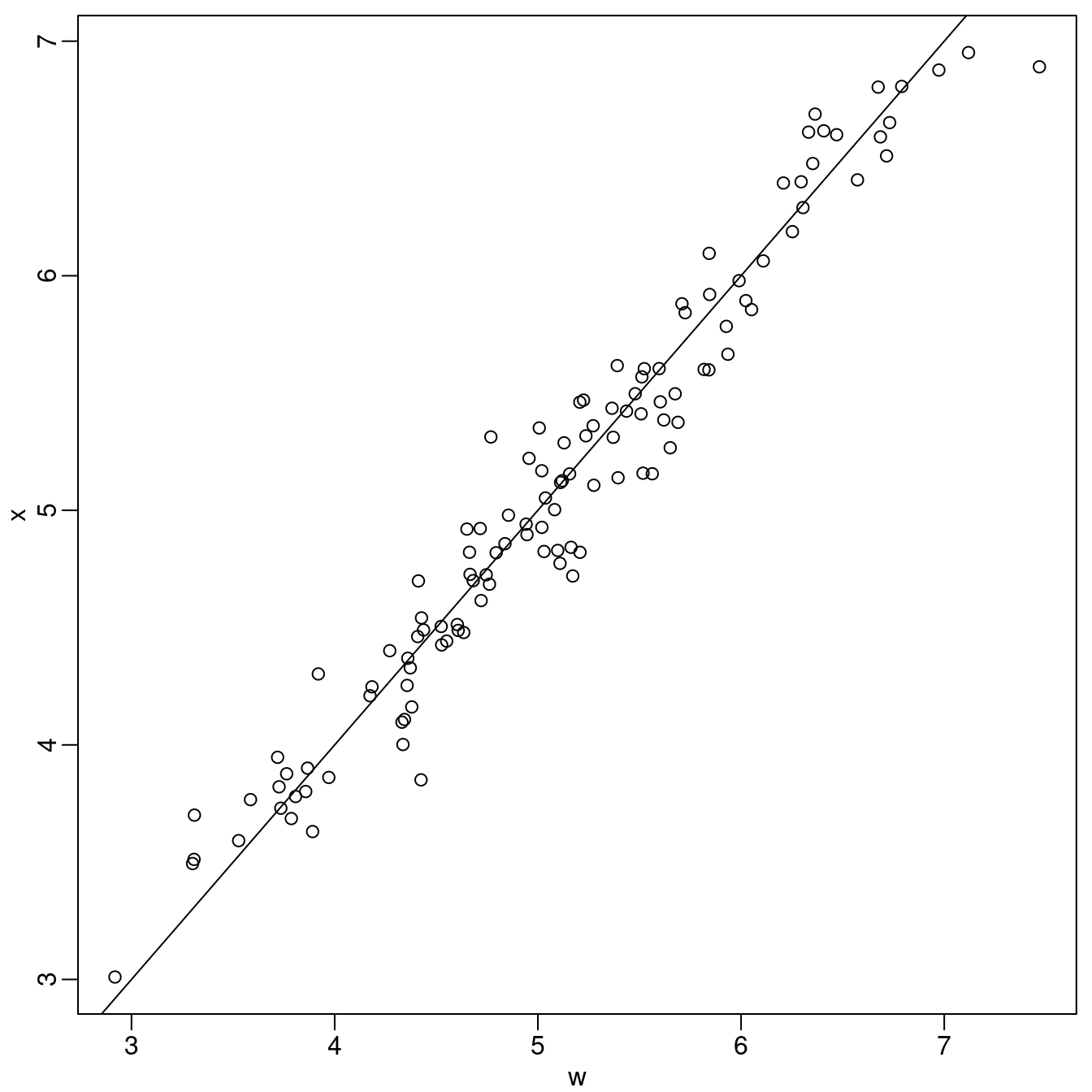

Figure 3.3: Simulated values of \(\mathbf{x}\) versus \(\mathbf{w}\).

Outcome \(\mathbf{y}\) is simulated as follows:

eta.y <- alpha.y + beta.x * x.y + v
set.seed(3)
yy <- rpois(n.y, exp(eta.y))

3.2.2 Model fitting

We build the mesh taking into account the value chosen for the ranges, range.v and range.m, of the spatial processes.

mesh <- inla.mesh.2d(rbind(loc.x, loc.y), 
  max.edge = min(range.m, range.v) * c(1 / 3, 1), 
  offset = min(range.m, range.v) * c(0.5, 1.5)) 

This mesh is made of 478 points. The same mesh will be considered to build the SPDE model for \(\mathbf{v}\) and \(\mathbf{m}\).

The projection matrices for the covariate and outcome locations are defined as follows:

Ax <- inla.spde.make.A(mesh, loc = loc.x)
Ay <- inla.spde.make.A(mesh, loc = loc.y)

For the parameters of the SPDE model, namely the practical range and the marginal standard deviation, we consider the PC-prior derived in Fuglstad et al. (2018), defined as:

spde <- inla.spde2.pcmatern(mesh = mesh,
  prior.range = c(0.5, 0.01), # P(practic.range < 0.5) = 0.01
  prior.sigma = c(1, 0.01)) # P(sigma > 1) = 0.01

In practice, the available data is \(w_j\), \(j={1, ..., n_x}\) and \(y_i\), \(i={n_x +1, ..., n_x+n_y}\). Thus, we need a model for \(\mathbf{x}\) that is able to compute (or predict) it at the outcome locations \(y_i\). From (3.1) we can write

\[\begin{align} \mathbf{0} = \alpha_x + \mathbf{m} - \mathbf{x}. \end{align}\]

Because \(\mathbf{m}\) is a GF, it can be defined over the entire area and used to predict \(\mathbf{x}\) at any point, particularly at the \(\mathbf{y}\) locations. This negative \(\mathbf{x}\) term is then copied into the \(\mathbf{y}\) linear predictor in order to estimate \(\beta\), using the copy feature.

To construct the stack for this model, we build one stack for each likelihood and then join them together. The data are supplied as a three column matrix where each column matches each likelihood in the inla() call. The first column contains the \(n_y\) “faked zeros”, while the other two columns contain . The effects should contain the intercept \(\alpha_x\), the index set for \(\mathbf{m}\) and an index from 1 to \(n_y\) to compute the \(-\mathbf{x}\) term at the \(\mathbf{y}\) locations. Since, \(\alpha_x\) and \(-\mathbf{x}\) are associated with each element of the “faked zero” observations, we group them in the same list element of the data stack. The index set for \(\mathbf{m}\) is another element on the effects list. These effects are associated respectively with the identity projector (or just a single number one) and the projector built earlier for the \(\mathbf{y}\) locations. As we will build more than one data stack, we use the to keep track of it. All of this can be written as follows:

stk.0 <- inla.stack(
  data = list(Y = cbind(rep(0, n.y), NA, NA)), 
  A = list(1, Ay),
  effects = list(data.frame(alpha.x = 1, x0 = 1:n.y, x0w = -1), 
    m = 1:spde$n.spde),  
  tag = 'dat.0') 

We now consider the \(\mathbf{w}\) data in the second column. We have that

\[\begin{align} \mathbf{w} \sim N(\mathbf{x} = \alpha_x + \mathbf{m}, \sigma_\epsilon^2\mathbf{I}), \end{align}\]

giving:

stk.x <- inla.stack(
  data = list(Y = cbind(NA, w.x, NA)), 
  A = list(1, Ax),
  effects = list(alpha.x = rep(1, n.x), m = 1:mesh$n), 
  tag = 'dat.x') 

To build the data stack for \(\mathbf{y}\) we need to include the terms for the intercept \(\alpha_y\), the index set for \(\mathbf{x}\) which will be copied from the “faked zero” observations model and the index for the \(\mathbf{v}\) term:

stk.y <- inla.stack(
  data = list(Y = cbind(NA, NA, yy)), 
  A = list(1, Ay),
  effects = list(data.frame(alpha.y = 1, x = 1:n.y),
    v = 1:mesh$n), 
  tag = 'dat.y')

We must supply only one formula for inla(), which should contain all the model terms. The terms in the right hand side of the formula that are not present in the data stack will just be ignored in the linear predictor for the corresponding data observations. The regression coefficient \(\beta\) is fitted with the copy feature, assuming a zero-mean Gaussian prior with precision 1. For the “faked zero” observations we assume for \(\alpha_x\) the default prior which is \(N(0, 1000)\). The SPDE model for \(\mathbf{m}\) is already defined, and \(\mathbf{x}\) gets an iid (independent and identically distributed) Gaussian random effect with low fixed precision. The \(\mathbf{x}\) is forced to be equal to \(\alpha_x - \mathbf{m}\) by considering a Gaussian likelihood with some (fixed) high precision and “faked zero” data.

form <- Y ~  0 + alpha.x + alpha.y + 
  f(m, model = spde) + f(v, model = spde) + 
  f(x0, x0w, model = 'iid', 
    hyper = list(prec = list(initial = -20, fixed = TRUE))) + 
  f(x, copy = 'x0', fixed = FALSE, 
    hyper = list(beta = list(prior = 'normal', param = c(0, 1)))) 
hfix <- list(hyper = list(prec = list(initial = 20,
  fixed = TRUE))) 

We consider a PC-prior for \(\sigma_\epsilon\) assuming P\((\sigma_\epsilon<0.2)=0.5\):

pprec <- list(hyper = list(prec = list(prior = 'pc.prec',
  param = c(0.2, 0.5))))

The model is then fitted stacking all the data previously defined:

stk <- inla.stack(stk.0, stk.x, stk.y) 
res <- inla(form, data = inla.stack.data(stk), 
  family = c('gaussian', 'gaussian', 'poisson'), 
  control.predictor = list(compute = TRUE, 
    A = inla.stack.A(stk)), 
  control.family = list(hfix, pprec, list())) 

3.2.3 Results

Table 3.4 shows the true values of model parameters used in the simulation as well as summaries of their posterior distributions. Figure 3.4 shows the posterior distribution of the regression parameters. We observe that for most of the cases, the true values of the parameters fall within the areas of high probability of the corresponding posterior distributions. The posterior distributions of the parameters of each random field are shown in Figure 3.5. The true values are also in the areas of high probability of their corresponding posterior marginal distributions.

Table 3.4: Summary of the posterior distributions of the parameters in the model.

Parameter	True	Mean	St. Dev.	2.5% quant.	97.5% quant.
\(\alpha_x\)	5.0	5.1457	0.3771	4.3692	5.8902
\(\alpha_y\)	2.0	2.3022	0.5282	1.2012	3.3164
\(\sigma_{\epsilon}\)	0.2	0.1882	0.0546	0.1004	0.3130
Range for m	3.0	2.8596	0.7157	1.8026	4.5823
Stdev for m	1.0	0.9949	0.1531	0.7455	1.3448
Range for v	3.0	4.0440	1.5762	2.0485	8.0682
Stdev for v	0.5	0.4699	0.1068	0.3034	0.7198
Beta for x	0.3	0.2573	0.0961	0.0714	0.4494

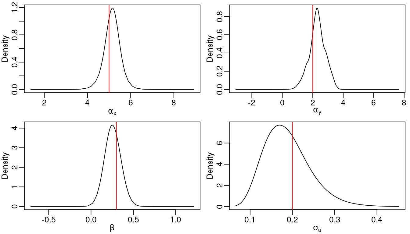
Figure 3.4: Posterior distribution of the intercepts, the regression coefficient and \(\sigma_{\epsilon}\). Vertical lines represent the actual value of the parameter used in the simulations.

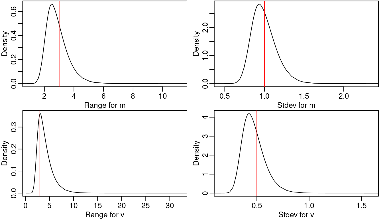
Figure 3.5: Posterior marginal distributions of the hyperparameters for both random fields. Vertical lines represent the actual value of the parameter used in the simulations.

Another interesting result is the prediction of the covariate at the response locations. Given that \(\mathbf{m}\) was simulated, we can assess how good the predictions for \(\mathbf{m}\) are at the \(\mathbf{x}\) and \(\mathbf{y}\) locations. We can project the posterior mean and standard deviations of \(\mathbf{m}\) at all the \(n_x\) and \(n_y\) locations:

mesh2locs <- rbind(Ax, Ay)
m.mu <- drop(mesh2locs %*% res$summary.ran$m$mean)
m.sd <- drop(mesh2locs %*% res$summary.ran$m$sd)

Then, we can approximate the 95% credible intervals for \(\mathbf{m}\) at each location, assuming a posterior normal distribution. This is shown in Figure 3.6, where the blue line represents the situation where the predicted value is equal to the simulated value.

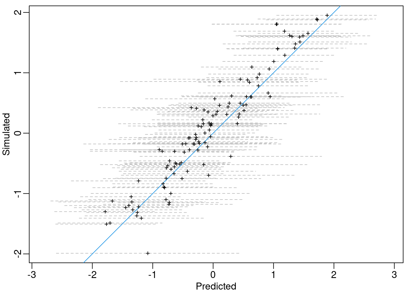
Figure 3.6: Simulated versus posterior mean of \(\mathbf{m}\) (\(+\)) and the approximated 95% credible intervals (grey dashed lines). The blue line represents the situation when the posterior mean is equal to the simulated values.

We visualize the expected value of \(\mathbf{m}\) and \(\mathbf{v}\) in Figure 3.7 with the following code:

# Create grid for projection
prj <- inla.mesh.projector(mesh, xlim = c(0, 10), ylim = c(0, 5))

# Settings for plotting device
par(mfrow = c(2, 1), mar = c(0.5, 0.5, 0.5, 0.5),
  mgp = c(1.5, 0.5, 0))

# Posterior mean of 'm'
book.plot.field(field = res$summary.ran$m$mean, projector = prj) 
points(loc.x, cex = 0.3 + (m - min(m))/diff(range(m)))
# Posterior mean of 'v'
book.plot.field(field = res$summary.ran$v$mean, projector = prj)
points(loc.y, cex = 0.3 + (v - min(v))/diff(range(v)))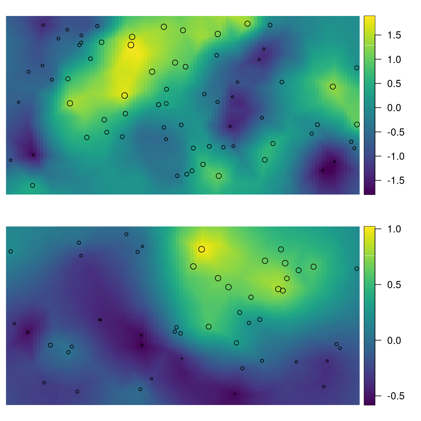

Figure 3.7: Posterior mean for \(\mathbf{m}\) and the \(\mathbf{x}\) locations plotted as points with size proportional to the simulated values for \(\mathbf{m}\) (top). Posterior mean for \(\mathbf{v}\) and the \(\mathbf{y}\) locations plotted as points with size proportional to the simulated values for \(\mathbf{v}\) (bottom).

3.3 Copying part of or the entire linear predictor

In this section we provide more insight into the technique of copying part of a linear predictor, which was used in both previous sections. In general, this is needed for all joint modeling.

Assume that data \(\mb{y}_1(\mb{s})\), \(\mb{y}_2(\mb{s})\) and \(\mb{y}_3(\mb{s})\) have been collected at location \(\mb{s}\). Also, consider the following models for the three types of observation:

\[\begin{eqnarray} \mb{y}_1(\mb{s}) & = & \beta_0 + \beta_1 \mb{x}(\mb{s}) + \mb{A}(\mb{s},\mb{s}_0)\mb{b}(\mb{s}_0) + \mb{\epsilon}_1(\mb{s}) \label{eq:y1obs} \\ \mb{y}_2(\mb{s}) & = & \beta_2(\beta_0 + \beta_1 \mb{x}(\mb{s})) + \mb{\epsilon}_2(\mb{s}) \label{eq:y2obs} \\ \mb{y}_3(\mb{s}) & = & \beta_3(\beta_0 + \beta_1 \mb{x}(\mb{s}) + \mb{A}(\mb{s},\mb{s}_0)\mb{b}(\mb{s}_0)) + \mb{\epsilon}_3(\mb{s}). \label{eq:y3obs} \end{eqnarray}\]

Here, the SPDE model is defined at the mesh nodes \(\mb{b}(\mb{s}_0)\) where \(\mb{A}(\mb{s},\mb{s}_0)\) is the projection matrix, and \(\mb{\epsilon}_j\), \(j=1,2,3\), are observation errors considered as zero mean Gaussians with variances \(\sigma^2_j\). In this setting, there is a different linear model for each outcome. Also, there is a common effect that is scaled from one linear predictor into another, where \(\beta_2\) and \(\beta_3\) are the scaling parameters.

We define the following model terms:

• \(\mb{\eta}_0(\mb{s}) = \beta_0 + \beta_1 \mb{x}(\mb{s})\)

• \(\mb{\eta}_1(\mb{s}) = \mb{\eta}_0(\mb{s}) + \mb{A}(\mb{s},\mb{s}_0)\mb{b}(\mb{s}_0)\)

• \(\mb{\eta}_2(\mb{s}) = \beta_2\mb{\eta}_0(\mb{s})\)

• \(\mb{\eta}_3(\mb{s}) = \beta_3\mb{\eta}_1(\mb{s})\)

We will show how to copy \(\mb{\eta}_0\) into \(\mb{\eta}_2\), and \(\mb{\eta}_1\) into \(\mb{\eta}_3\), in order to estimate \(\beta_2\) and \(\beta_3\). Furthermore, all the three observation vectors, \(\mb{y}_1\), \(\mb{y}_2\) and \(\mb{y}_3\), are assumed to be observed at the same locations.

3.3.1 Generating the data

The set of parameters in the model for \(\beta_j\), \(j=0,1,2,3\), is defined as follows:

beta0 = 5
beta1 = 1
beta2 = 0.5
beta3 = 2

Then, the standard deviations of the error terms are defined as:

s123 <- c(0.1, 0.05, 0.15)

For the \(\mb{b}(\mb{s})\) process, a Matérn covariance function with \(\kappa_b\), \(\sigma^2_b\) and \(\nu=1\) (fixed) is considered, so that the following parameters are defined:

kappab <- 10
sigma2b <- 1

To obtain a realization of the spatial process, a set of locations is considered as follows:

n <- 50
loc <- cbind(runif(n), runif(n))

As in previous sections, the sample from the Matérn process will be obtained using function book.rMatern (see Section 2.1.3).

b <- book.rMatern(n = 1, coords = loc, 
  range = sqrt(8) / 10, sigma = 1)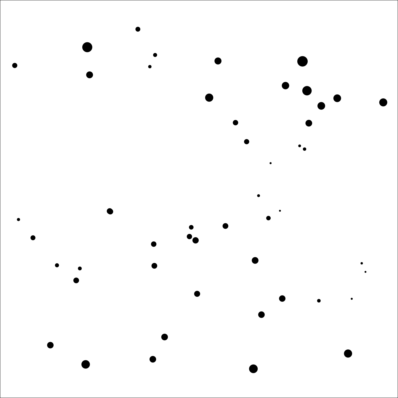

Figure 3.8: Locations of the simulated dataset. Point size is proportional to the value of the underlying Matérn process.

We plot this sample in Figure 3.8. We simulate a covariate as follows:

x <- sqrt(3) * runif(n, -1, 1) 

Then, the required linear predictors are computed:

eta1 <- beta0 + beta1 * x + b
eta2 <- beta2 * (beta0 + beta1 * x)
eta3 <- beta3 * eta1

Finally, the observations are obtained:

y1 <- rnorm(n, eta1, s123[1])
y2 <- rnorm(n, eta2, s123[2])
y3 <- rnorm(n, eta3, s123[3])

3.3.2 The fake zero trick for fitting this model

There is more than one way to fit this model using the INLA package. The main point is the need to compute \(\mb{\eta}_0(\mb{s}) = \beta_0 + \beta_1 \mb{x}(\mb{s})\) and \(\mb{\eta}_1(\mb{s}) = \beta_0 + \beta_1 \mb{x}(\mb{s}) + \mb{A}(\mb{s},\mb{s}_0)\mb{b}(\mb{s})\) from the first observation equation in order to copy it to the second and third observation equations. So, a model that computes \(\mb{\eta}_0(\mb{s})\) and \(\mb{\eta}_1(\mb{s})\) explicitly needs to be defined.

The way we choose is to minimize the size of the graph generated by the model (Rue et al. 2017). First, the following equations are considered:

\[\begin{eqnarray} \mb{0}(\mb{s}) & = & \mb{A}(\mb{s},\mb{s}_0)\mb{b}(\mb{s}_0) + \mb{\eta}_0(\mb{s}) + \mb{\epsilon}_1(\mb{s}) - \mb{y}_1(\mb{s}) \label{eq:eta0} \\ \mb{0}(\mb{s}) & = & \mb{\eta}_1(\mb{s}) + \mb{\epsilon}_1(\mb{s}) - \mb{y}_1(\mb{s}) \label{eq:eta1} \end{eqnarray}\]

where only \(\mb{A}(\mb{s},\mb{s}_0)\), \(\mb{x}(\mb{s})\) and \(\mb{y}_1(\mb{s})\) are known. For the \(\mb{\eta}_0(\mb{s})\) and \(\mb{\eta}_2(\mb{s})\) terms, we assume independent and identically distributed (i.e., iid) models with low fixed precision. With this fixed high variance, each element in \(\mb{\eta}_0(\mb{s})\) and \(\mb{\eta}_1(\mb{s})\) can take any value.

However, these values will be forced to be \(\beta_0 + \beta_1 \mb{x}(\mb{s})\) and \(\beta_0 + \beta_1 \mb{x}(\mb{s}) + \mb{A}(\mb{s},\mb{s}_0)\mb{b}(\mb{s}_0)\) by considering a Gaussian likelihood for the “faked zero” observations with a high fixed precision value (i.e., a low fixed likelihood variance). For details and examples of this approach see Section 3.2, and Ruiz-Cárdenas, Krainski, and Rue (2012), Martins et al. (2013) and Chapter 8 in Blangiardo and Cameletti (2015).

Since three Gaussian likelihoods are considered for the observed data, three error terms can be included in the linear predictors and can fix the likelihood precisions to high values. With this setting, the three Gaussian likelihoods with high fixed precisions become a single Gaussian likelihood.

3.3.3 Fitting the model

In order to fit the \(\mb{b}(\mb{s})\) term, we define a SPDE Matérn model. For this, the first step is to set a mesh:

mesh <- inla.mesh.2d(
  loc.domain = cbind(c(0, 1, 1, 0), c(0, 0, 1, 1)),
  max.edge = c(0.1, 0.3), offset = c(0.05, 0.35), cutoff = 0.05)

Next, the projection matrix is defined:

As <- inla.spde.make.A(mesh, loc)

Then, the SPDE model is defined:

spde <- inla.spde2.pcmatern(mesh, alpha = 2, 
  prior.range = c(0.05, 0.01),
  prior.sigma = c(1, 0.01))

The data have to be organized using the inla.stack() function. The data stack for the first observation vector is:

stack1 <- inla.stack(
  data = list(y = y1), 
  A = list(1, As, 1),
  effects = list(
    data.frame(beta0 = 1, beta1 = x),
    s = 1:spde$n.spde,
    e1 = 1:n),
  tag = 'y1')

Here, the e1 term will be used to fit \(\mb{\epsilon}_1\). Similarly, the data stack for the first “faked zero” observations is:

stack01 <- inla.stack(
  data = list(y = rep(0, n), offset = -y1),
  A = list(As, 1),
  effects = list(s = 1:spde$n.spde,
    list(e1 = 1:n, eta1 = 1:n)),
  tag = 'eta1')

Here, the data stack includes minus the first observation vector as an offset. The stack for the second “faked zero” observation is:

stack02 <- inla.stack(
  data = list(y = rep(0, n), offset = -y1),
  effects = list(list(e1 = 1:n, eta2 = 1:n)),
  A = list(1),
  tag = 'eta2')

The stack for the second vector of observations now considers an index set to compute the \(\mb{\eta}_1\) term copied from the first “faked zero” observations:

stack2 <- inla.stack(
  data = list(y = y2),
  effects = list(list(eta1c = 1:n, e2 = 1:n)), 
  A = list(1),
  tag = 'y2')

In a similar way, the third observation stack also includes an index set to compute the \(\mb{\eta}_2\) term copied from the second “faked zero” observations:

stack3 <- inla.stack(
  data = list(y = y3), 
  effects = list(list(eta2c = 1:n, e3 = 1:n)),
  A = list(1),
  tag = 'y3')

Once all the different data stacks have been defined, they are combined into a new one that will be used to fit the model:

stack <- inla.stack(stack1, stack01, stack02, stack2, stack3)

We use the default priors for most of the parameters. For the three variance errors in the observations PC-priors will be set as follows:

pcprec <- list(prec = list(prior = 'pcprec',
  param = c(0.5, 0.1)))

formula123 <- y ~ 0 + beta0 + beta1 + 
  f(s, model = spde) + f(e1, model = 'iid', hyper = pcprec) +
  f(eta1, model = 'iid',
    hyper = list(prec = list(initial = -10, fixed = TRUE))) + 
  f(eta2, model = 'iid',
    hyper = list(prec = list(initial = -10, fixed = TRUE))) + 
  f(eta1c, copy = 'eta1', fixed = FALSE) +
  f(e2, model = 'iid', hyper = pcprec) +
  f(eta2c, copy = 'eta2', fixed = FALSE) +
  f(e3, model = 'iid', hyper = pcprec)

Finally, the model is fitted:

res123 <- inla(formula123,
  data = inla.stack.data(stack),
  offset = offset,
  control.family = list(list(
    hyper = list(prec = list(initial = 10, fixed = TRUE)))),
  control.predictor = list(A = inla.stack.A(stack)))

3.3.4 Model results

A summary of the fixed effects \(\beta_0\) and \(\beta_1\), as well as the \(\beta_2\) and \(\beta_3\) parameters is available in Table 3.5.

Table 3.5: Posterior modes of some of the model parameters.

Parameter	True	Mean	St. Dev.	2.5% quant.	97.5% quant.
\(\beta_0\)	5.0	5.2824	0.0489	5.2116	5.3722
\(\beta_1\)	1.0	0.9864	0.0253	0.9365	1.0361
Beta for eta1c	0.5	0.4923	0.0187	0.4658	0.5359
Beta for eta2c	2.0	2.0109	0.0081	1.9963	2.0281

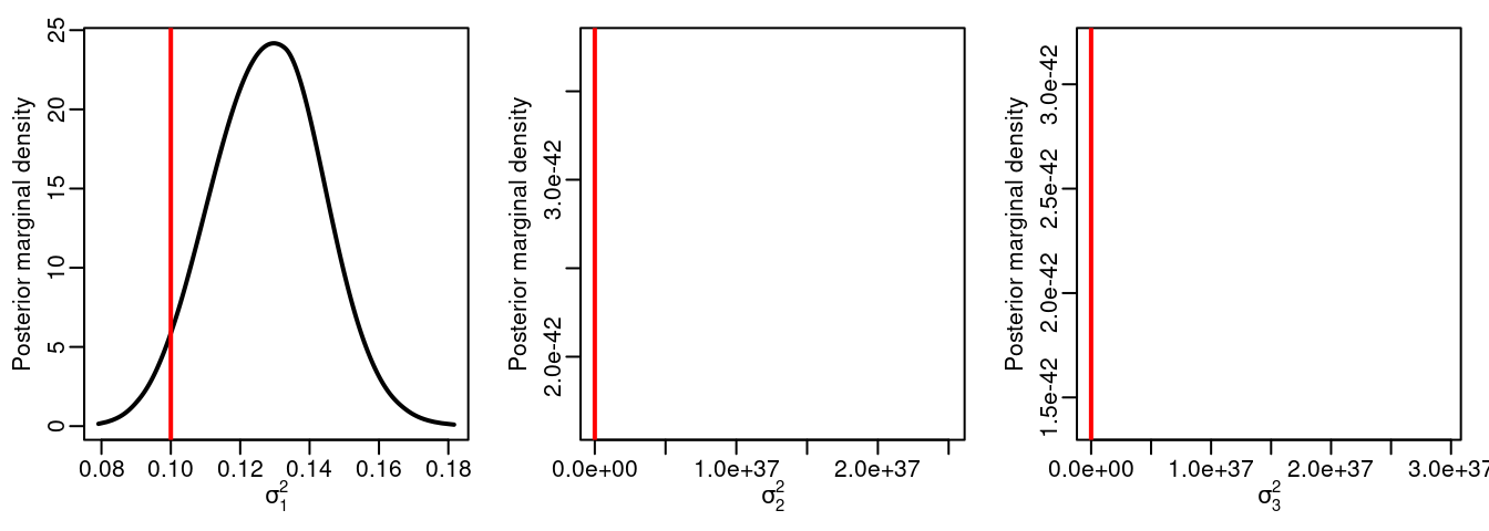
Figure 3.9: Observation error standard deviations. Vertical lines represent the actual values of the parameters.

Figure 3.9 shows the posterior marginal distribution of the standard deviation for \(\mb{\epsilon}_1\), \(\mb{\epsilon}_2\) and \(\mb{\epsilon}_3\). Similarly, Figure 3.10 shows the posterior marginals of the random field parameters.

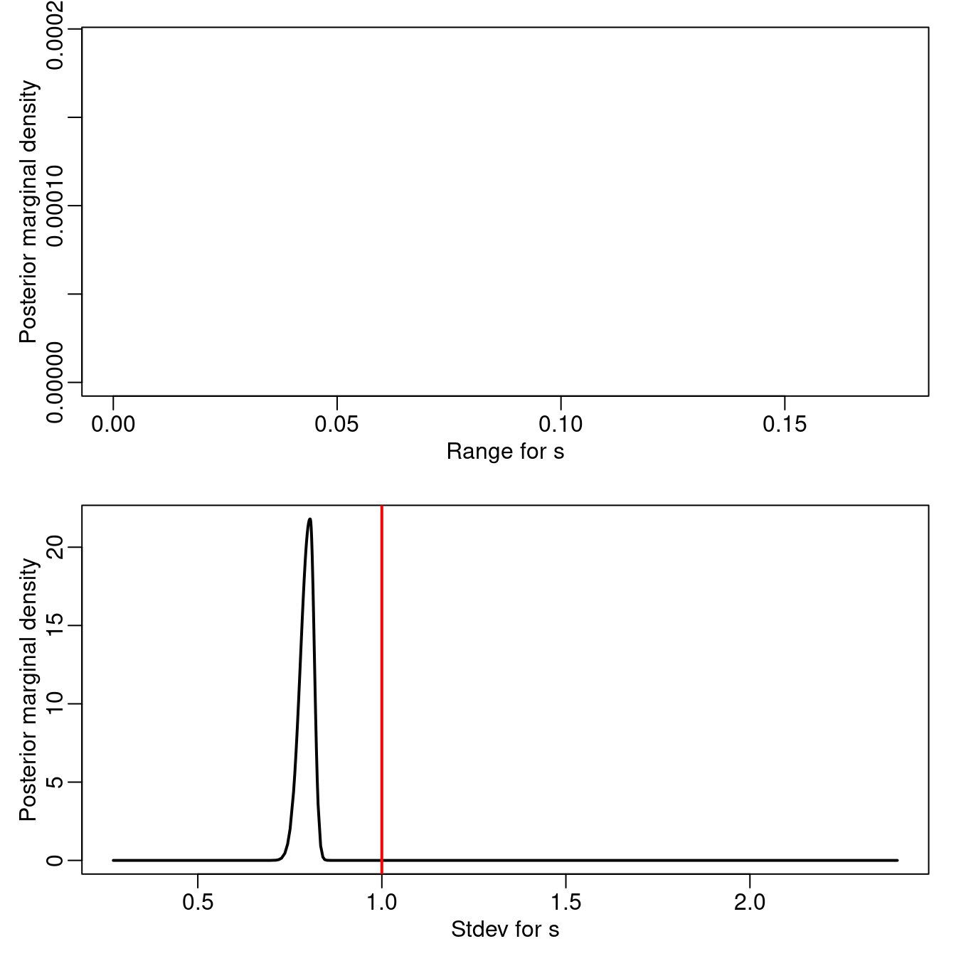
Figure 3.10: Posterior marginal distributions for the random field parameters. Vertical lines represent the actual values of the parameters.

References

Blangiardo, M., and M. Cameletti. 2015. Spatial and SpatioTemporal Bayesian Models with R-INLA. Chichester, UK: John Wiley & Sons, Ltd.

Fuglstad, G-A., D. Simpson, F. Lindgren, and H. Rue. 2018. “Constructing Priors That Penalize the Complexity of Gaussian Random Fields.” Journal of the American Statistical Association to appear. https://doi.org/10.1080/01621459.2017.1415907.

Gelfand, A. E., A. M. Schmidt, and C. F. Sirmans. 2002. “Multivariate Spatial Process Models: Conditional and Unconditional Bayesian Approaches Using Coregionalization.” Center for Real Estate and Urban Economic Studies, University of Connecticut.

Martins, T. G., D. Simpson, F. Lindgren, and H. Rue. 2013. “Bayesian computing with INLA: New features.” Computational Statistics & Data Analysis 67 (0): 68–83. https://doi.org/10.1016/j.csda.2013.04.014.

Muff, S., A. Riebler, L. Held, H. Rue, and P. Saner. 2014. “Bayesian Analysis of Measurement Error Models Using Integrated Nested Laplace Approximations.” Journal of the Royal Statistical Society: Series C 64 (2): 231–52.

Rue, H., A. I. Riebler, S. H. Sørbye, J. B. Illian, D. P. Simpson, and F. K. Lindgren. 2017. “Bayesian Computing with INLA: A Review.” Annual Review of Statistics and Its Application 4: 395–421.

Ruiz-Cárdenas, R., E. T. Krainski, and H. Rue. 2012. “Direct Fitting of Dynamic Models Using Integrated Nested Laplace Approximations — INLA.” Computational Statistics & Data Analysis 56 (6): 1808–28. https://doi.org/http://dx.doi.org/10.1016/j.csda.2011.10.024.

Schmidt, A. M., and A. E. Gelfand. 2003. “A Bayesian Coregionalization Approach for Multivariate Pollutant Data.” Journal of Geographysical Research 108 (D24).