Chapter 2 Introduction to spatial modeling
2.1 Introduction
In this section, a brief summary of continuous spatial processes will be provided, and the Stochastic Partial Differential Equations - SPDE approach -
as proposed in Lindgren, Rue, and Lindström (2011) will be summarized intuitively.
Provided that a Gaussian spatial process with Matérn covariance is a solution to SPDE’s
of the form presented in Lindgren, Rue, and Lindström (2011), we will give an
intuitive presentation of the main results of this link.
The Matérn covariance function is probably the most used one in geostatistics.
Therefore, the approach in Lindgren, Rue, and Lindström (2011) is useful
because the Finite Element Method (FEM) was used to build a GMRF
(Rue and Held 2005) representation and is available for practitioners
through the INLA package.
A recent review of spatial models in INLA can be found in Bakka et al. (2018).
2.1.1 Spatial variation
A point-referenced dataset is made up of any data measured at known locations. These locations may be in any coordinate reference system, most often longitude and latitude. Point-referenced data are common in many areas of science. This type of data appears in mining, climate modeling, ecology, agriculture and other fields. If the influence of location needs to be incorporated into a model, then a model for geo-referenced data is required.
As shown in Chapter 1, a regression model can be built using the coordinates of the data as covariates to describe the spatial variation of the variable of interest. In many cases, a non-linear function based on the coordinates will be necessary to adequately describe the effect of the location. For example, basis functions on the coordinates can be used as covariates in order to build a smooth function. This specification explicitly models the spatial trend on the mean.
Alternatively, it may be more natural to explicitly model the variation of the outcome considering that it may be similar at nearby locations. The first law of geography asserts: ``Everything is related to everything else, but near things are more related than distant things’’ (Tobler 1970). This means that the proposed model should have the property that an observation is more correlated with an observation close in space than with another observation that has been collected further away.
In spatial statistics it is common to formulate mixed-effects regression models in which the linear predictor is made of a trend plus a spatial variation (Haining 2003). The trend usually is composed of fixed effects or some smooth terms on covariates, while the spatial variation is usually modeled using correlated random effects. Spatial random effects often model (residual) small scale variation and this is the reason why these models can be regarded as models with correlated errors.
Models that account for spatial dependence may be defined according to whether locations are areas (cities or countries, for example) or points. For a review of models for different types of spatial data see, for example, Haining (2003) and Cressie and Wikle (2011).
The case of areal data (also known as lattice data) is often tackled by the use of generalized linear mixed-effects models given that variables are measured at a discrete number of locations. Given a vector of observations \(\mathbf{y} = (y_1, \ldots, y_n)\) from \(n\) areas, the model can be represented as
\[ y_i|\mu_i,\mathbf{\theta} \sim f(\mu_i; \mathbf{\theta}) \]
\[ g(\mu_i) = X_i \mathbf{\beta} + u_i;\ i = 1, \ldots, n \]
Here, \(f(\mu_i; \mathbf{\theta})\) is a distribution with mean \(\mu_i\) and hyperparameters \(\mathbf{\theta}\). The function \(g(\cdot)\) links the mean of each observation to a linear predictor on a vector of covariates \(X_i\) with coefficients \(\mathbf{\beta}\). The terms \(u_i\) represent random effects, distributed usually using a Gaussian multivariate distribution with zero mean and precision matrix \(\tau Q\).
While \(\tau\) is a precision hyperparameter, the structure of the precision matrix is given by the matrix \(Q\) and is defined in a way that captures the spatial correlation in the data. For lattice data, \(Q\) is often based on the adjacency matrix that represents the neighborhood structure of the areas where data has been collected. This adjacency is illustrated in Figure 2.1, where the adjacency structure of the 100 counties in North Carolina is represented by a graph. This graph can be represented using a \(100\times 100\) matrix \(W\) with \(1\) at entry \((i, j)\) if counties \(i\) and \(j\) are neighbors and 0 otherwise.
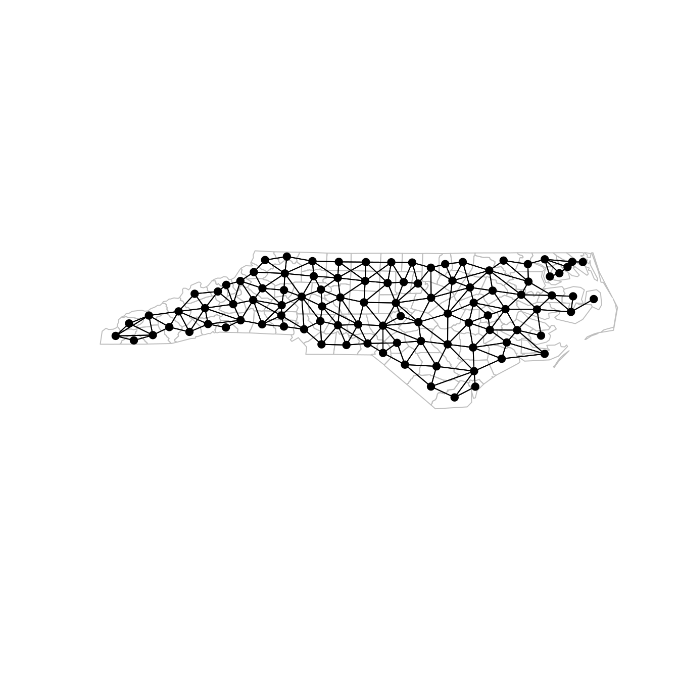
Figure 2.1: Counties in North Carolina and their neighborhood structure.
A simple way to define spatially correlated random effects using the adjacency matrix \(W\) is to take \(Q = I - \rho W\), where \(I\) is the identity matrix and \(\rho\) is a spatial autocorrelation parameter. This is known as a CAR specification (Schabenberger and Gotway 2004). Nevertheless, there are other ways to exploit \(W\) to define \(Q\) to model spatial autocorrelation. See, for example, Haining (2003), Cressie and Wikle (2011) or Banerjee, Carlin, and Gelfand (2014).
Spatial data that is observed at specific locations is usually divided in two particular cases, depending on whether locations are fixed (geostatistics or point-referenced data) or random (point process). Note that in both cases the underlying spatial process will be defined at every point of the study region and not at a discrete number of locations (as in the case of lattice data). A general description of model-based geostatistics can be found in Diggle and Ribeiro Jr. (2007). Point pattern analysis is thoroughly described in Illian et al. (2008), Diggle (2013) and Baddeley, Rubak, and Turner (2015), for example.
Modeling and analyzing data observed at specific locations is the primary object of this book and these two cases will be considered in more detail. Next, Gaussian random fields to model continuous spatial processes will be introduced.
2.1.2 The Gaussian random field
To introduce some notation, let \(\mathbf{s}\) be any location in a study area \(\mathbf{D}\) and let \(U(\mathbf{s})\) be the random (spatial) effect at that location. \(U(\mathbf{s})\) is a stochastic process, with \(\mathbf{s}\in \mathbf{D}\), where \(\mathbf{D}\subset \mathbb{R}^d\). Suppose, for example, that \(\mathbf{D}\) is a country and data have been measured at geographical locations, over \(d=2\) dimensions within this country.
We denote by \(u(\textbf{s}_i)\), \(i=1,2,\ldots,n\) a realization of \(U(\mathbf{s})\) at \(n\) locations. It is commonly assumed that \(u(\mathbf{s})\) has a multivariate Gaussian distribution. If \(U(\mathbf{s})\) is assumed to be continuous over space, then it is a continuously-indexed Gaussian field (GF). This implies that it is possible to collect these data at any finite set of locations within the study region. To complete the specification of the distribution of \(u(\mathbf{s})\), it is necessary to define its mean and covariance.
A very simple option is to define a correlation function based only on the Euclidean distance between locations. This assumes that given two pairs of points separated by the same distance \(h\), they will have the same degree of correlation; Abrahamsen (1997) presents Gaussian random fields and correlation functions.
Now suppose that data \(y_i\) have been observed at locations \(\textbf{s}_i\), \(i=1,...,n\). If an underlying GF generated these data, the parameters of this process can be fitted by considering \(y(\textbf{s}_i) = u(\textbf{s}_i)\), where observation \(y(\textbf{s}_i)\) is assumed to be a realization of the GF at the location \(\textbf{s}_i\). If it is further assumed that \(y(\textbf{s}_i) = \mu + u(\textbf{s}_i)\), then there is one more parameter to estimate. It is worth mentioning that the distribution of \(u(\mathbf{s})\) at a finite number of points is considered a realization of a multivariate Gaussian distribution. In this case, the likelihood function is the multivariate Gaussian distribution with covariance \(\Sigma\).
In many situations it is assumed that there is an underlying GF that cannot be directly observed. Instead, observations are data with a measurement error \(e_i\), i.e.,
\[\begin{equation} \tag{2.1} y(\textbf{s}_i) = u(\textbf{s}_i) + e_i . \end{equation}\]
It is common to assume that \(e_i\) is independent of \(e_j\) for all \(i\neq j\) and \(e_i\) follows a Gaussian distribution with zero mean and variance \(\sigma_e^2\). This additional parameter, \(\sigma_e^2\), is also known as the “nugget effect” in geostatistics. The covariance of the marginal distribution of \(y(\mathbf{s})\) at a finite number of locations is \(\Sigma_y = \Sigma + \sigma^2_e\mathbf{I}\). This is a short extension of the basic GF model, and gives one additional parameter to estimate. For more details about this geostatistics model see, for example, Diggle and Ribeiro Jr. (2007).
The spatial process \(u(\textbf{s})\) if often assumed to be stationary and isotropic. A spatial process is stationary if its statistical properties are invariant under translation; i.e., they are the same at any point of the study region. Isotropy means that the process is invariant under rotation; i.e., their properties do not change regardless of the direction we move around the study region. Stationary and isotropic spatial process play an important role in spatial statistics, as they have desirable properties, such as a constant mean and the fact that the covariance between any two points only depends on their distance and not on their relative position. See, for example, Cressie and Wikle (2011), Section 2.2, for more details about these properties.
The usual way to evaluate the likelihood function, which is just a multivariate Gaussian density for the model in Equation (2.1), usually considers a Cholesky factorization of the covariance matrix (see, for example, Rue and Held 2005). Because this matrix is dense, this is an operation of order \(O(n^3)\), so this is a “big \(n\) problem”. Some software for geostatistical analysis uses an empirical variogram to fit the parameters of the correlation function. However, this option does not make any assumptions about a likelihood function for the data or uses a multivariate Gaussian distribution for the spatially structured random effect. A good description of these techniques is available in Cressie (1993).
To model spatial dependence with non-Gaussian data, it is usual to assume a likelihood for the data conditional on an unobserved random effect, which is a GF. Such spatial mixed effects models fall under the model-based geostatistics approach (Diggle and Ribeiro Jr. 2007). It is possible to describe the model in Equation (2.1) within a larger class of models: hierarchical models. Suppose that observations \(y_i\) have been obtained at locations \(\textbf{s}_i\), \(i=1,...,n\). The starting model is
\[\begin{equation} \tag{2.2} \begin{array}{rcl} y_i|\mathbf{\beta},u_i,\mathbf{F}_i,\phi & \sim & f(y_i|\mu_i,\phi) \\ \mathbf{u}|\mathbf{\theta} & \sim & GF(0, \Sigma) \end{array} \end{equation}\]
where \(\mu_i = h(\mathbf{F}_i^{T}\mathbf{\beta} + u_i)\). Here, \(\mathbf{F}_i\) is a matrix of covariates with associated coefficients \(\mathbf{\beta}\), \(\mathbf{u}\) is a vector of random effects and \(h(\cdot)\) is a function mapping the linear predictor \(\mathbf{F}_i^{T}\mathbf{\beta} + u_i\) to E\((y_i) = \mu_i\). In addition, \(\mathbf{\theta}\) are parameters for the random effect and \(\phi\) is a dispersion parameter of the distribution of the data \(f(\cdot)\), which is assumed to be in the exponential family.
To write the GF (with the Gaussian noise as a nugget effect), \(y_i\) is assumed to have a Gaussian distribution (with variance \(\sigma_e^2\)), \(\mathbf{F}_i^{T}\mathbf{\beta}\) is replaced by \(\beta_0\) and \(\mathbf{u}\) is modeled as a GF. Furthermore, it is possible to consider a multivariate Gaussian distribution for the random effect but it is seldom practical to use the covariance directly for model-based inference. This is shown in Equation (2.3).
\[\begin{equation} \tag{2.3} \begin{array}{rcl} y_i|\mu_i,\sigma_e &\sim& N(y_i|\mu_i,\sigma_e^2) \\ \mu_i &=&\beta_0 + u_i\\ \mathbf{u}|\theta &\sim& GF(0, \Sigma) \end{array} \end{equation}\]
As mentioned in Section 2.1.1, in the analysis of areal data there are models specified by conditional distributions that imply a joint distribution with a sparse precision matrix. These models are called Gaussian Markov random fields (GMRF) and a good reference is Rue and Held (2005). It is computationally easier to make Bayesian inference when a GMRF is used than when a GF is used, because the computational cost of working with a sparse precision matrix in GMRF models is (typically) \(O(n^{3/2})\) in \(\mathbb{R}^2\). This makes it easier to conduct analyses with big \(n\).
This basic hierarchical model can be extended in many ways, and some extensions will be considered later. When the general properties of the GF are known, all the practical models that contain, or are based on this random effect can be studied.
2.1.3 The Matérn covariance
A very popular correlation function is the Matérn correlation function. It has a scale parameter \(\kappa>0\) and a smoothness parameter \(\nu>0\). For two locations \(\textbf{s}_i\) and \(\textbf{s}_j\), the stationary and isotropic Matérn correlation function is:
\[ Cor_M(U(\textbf{s}_i), U(\textbf{s}_j)) = \frac{2^{1-\nu}}{\Gamma(\nu)} (\kappa \parallel \textbf{s}_i - \textbf{s}_j\parallel)^\nu K_\nu(\kappa \parallel \textbf{s}_i - \textbf{s}_j \parallel) \]
where \(\parallel . \parallel\) denotes the Euclidean distance and \(K_\nu\) is the modified Bessel function of the second kind. The Matérn covariance function is \(\sigma^2_u Cor_M(U(\textbf{s}_i), U(\textbf{s}_j))\), where \(\sigma^2_u\) is the marginal variance of the process.
If \(u(\mathbf{s})\) is a realization from \(U(\mathbf{s})\) at \(n\) locations, \(\textbf{s}_1, ..., \textbf{s}_n\), its joint covariance matrix can be easily defined as each entry of this joint covariance matrix \(\Sigma\) is \(\Sigma_{i,j} = \sigma_u^2 Cor_M(u(\textbf{s}_i), u(\textbf{s}_j))\). It is common to assume that \(U(.)\) has a zero mean. Hence, we have now completely defined a multivariate distribution for \(u(\mathbf{s})\).
To gain a better understanding about the Matérn correlation, samples can be drawn from the GF process. A sample \(\mathbf{u}\) is drawn considering \(\mathbf{u} = \mathbf{R}^\top \mathbf{z}\) where \(\mathbf{R}\) is the Cholesky decomposition of the covariance at \(n\) locations (see below); i.e., the covariance matrix is equal to \(\mathbf{R}^\top \mathbf{R}\) with \(\mathbf{R}\) an upper triangular matrix, and \(\mathbf{z}\) is a vector with \(n\) samples drawn from a standard Gaussian distribution. It implies that \(\textrm{E}(\mathbf{u}) = \textrm{E}(\mathbf{R^\top z}) = \mathbf{R}^\top \textrm{E}(\mathbf{z}) = \mathbf{0}\) and \(\textrm{Var}(\mathbf{u}) = \mathbf{R}^\top\textrm{Var}(\mathbf{z})\mathbf{R}=\mathbf{R}^\top\mathbf{R}\).
Two useful functions to sample from a GF are defined below:
# Matern correlation
cMatern <- function(h, nu, kappa) {
  ifelse(h > 0, besselK(h * kappa, nu) * (h * kappa)^nu /
    (gamma(nu) * 2^(nu - 1)), 1)
}

# Function to sample from zero mean multivariate normal
rmvnorm0 <- function(n, cov, R = NULL) {
  if (is.null(R))
    R <- chol(cov)

  return(crossprod(R, matrix(rnorm(n * ncol(R)), ncol(R))))
}
Function cMatern() computes the Matérn covariance of two points at distance
h, which requires additional parameters nu and kappa. Function
rmvnorm0() computes n samples from a multivariate Gaussian distribution
using the Cholesky decomposition, which needs the covariance matrix cov or
the upper triangles matrix R from a Cholesky decomposition.
Hence, given \(n\) locations, function cMatern() can be used to compute the
Matérn covariance, and function rmvnorm0() can be used to draw samples. These steps are
collected into the function book.rMatern, which is available in the file
spde-book-functions.R. This file is available from the website of this
book.
In order to simplify the visualization of the properties of continuous spatial processes with a Matérn covariance, a set of \(n=249\) locations in the one-dimensional space from 0 to \(25\) will be considered.
# Define locations and distance matrix
loc <- 0:249 / 25
mdist <- as.matrix(dist(loc))
Four values for the smoothness parameter \(\nu\) will be considered. The values for the \(\kappa\) parameter were determined from the range expression \(\sqrt{8\nu}/\kappa\), which is the distance that gives correlation near \(0.14\). By combining the four values for \(\nu\) with two range values, there are eight parameter configurations.
The values of the different parameters \(\nu\), range and \(\kappa\) are created as follows:
# Define parameters
nu <- c(0.5, 1.5, 2.5, 5.5)
range <- c(1, 4)
Next, the different combinations of the parameters are put together in a
matrix:
# Covariance parameter scenarios
params <- cbind(nu = rep(nu, length(range)),
  range = rep(range, each = length(nu)))
Sampled values depend on the covariance matrix and the noise considered for the
standard Gaussian distribution. In the following example, five vectors of size
\(n\) are drawn from the standard Gaussian distribution. These five standard
Gaussian observations, z in the code below, were the same across the eight
parameter configurations in order to keep track of what the different parameter
configurations are doing.
# Sample error
set.seed(123)
z <- matrix(rnorm(nrow(mdist) * 5), ncol = 5)
Therefore, there is a set of \(40\) different realizations, five for each parameter configuration:
# Compute the correlated samples
# Scenarios (i.e., different set of parameters)
yy <- lapply(1:nrow(params), function(j) {
  param <- c(params[j, 1], sqrt(8 * params[j, 1]) / params[j, 2],
    params[j, 2])
  v <- cMatern(mdist, param[1], param[2])

  # fix the diagonal to avoid numerical issues
  diag(v) <- 1 + 1e-9

  # Parameter scenario and computed sample
  return(list(params = param, y = crossprod(chol(v), z)))
})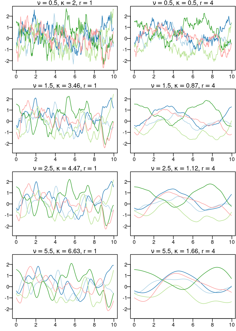
Figure 2.2: Five samples from the one-dimensional Matérn correlation function for two different range values (each column of plots) and four different values for the smoothness parameter (each line of plots).
These samples are shown in the eight plots in Figure 2.2. One important point to observe here is the main spatial trend in the samples, as it seems not to depend on the smoothness parameter \(\nu\). In order to appreciate the main trend, consider one of the five samples (i.e., one of the colors). Then, compare the curves for different values of the smoothness parameter. If noise is added to the smoothest curve, and the resulting curve is compared to the other curves fitted using different smoothness parameters, it is difficult to disentangle what is due to noise from what is due to smoothness. Therefore, in practice, the smoothness parameter is usually fixed and a noise term is added.
2.1.4 Simulation of a toy data set
Now, a sample from the model in Equation (2.1) will be drawn and it
will be used in Section 2.3. A set of \(n=100\) locations in
the unit square will be considered. This sample will have a higher density of
locations in the bottom left corner than in the top right corner. The R code
to do this is:
n <- 200
set.seed(123)
pts <- cbind(s1 = sample(1:n / n - 0.5 / n)^2,
  s2 = sample(1:n / n - 0.5 / n)^2)
To get a (lower triangular) matrix of distances, the dist() function
can be used as follows:
dmat <- as.matrix(dist(pts))The chosen parameters for the Matérn covariance are \(\sigma^2_u=5\), \(\kappa=7\) and \(\nu=1\). The mean is set to be \(\beta_0=10\) and the nugget parameter is \(\sigma^2_e=0.3\). These values are declared using:
beta0 <- 10
sigma2e <- 0.3
sigma2u <- 5
kappa <- 7
nu <- 1
Now, a sample is obtained from a multivariate distribution
with constant mean equal to \(\beta_0\) and
covariance \(\sigma^2_e\mathbf{I} + \Sigma\), which is the
marginal covariance of the observations. \(\Sigma\) is the Matérn covariance
of the spatial process, mcor in the code below.
mcor <- cMatern(dmat, nu, kappa)
mcov <- sigma2e * diag(nrow(mcor)) + sigma2u * mcor
Next, the sample is obtained by considering the Cholesky factor times a unit variance noise and add the mean:
R <- chol(mcov)
set.seed(234)
y1 <- beta0 + drop(crossprod(R, rnorm(n)))
Figure 2.3 shows these simulated data in a graph of the locations where the size of the points is proportional to the simulated values.
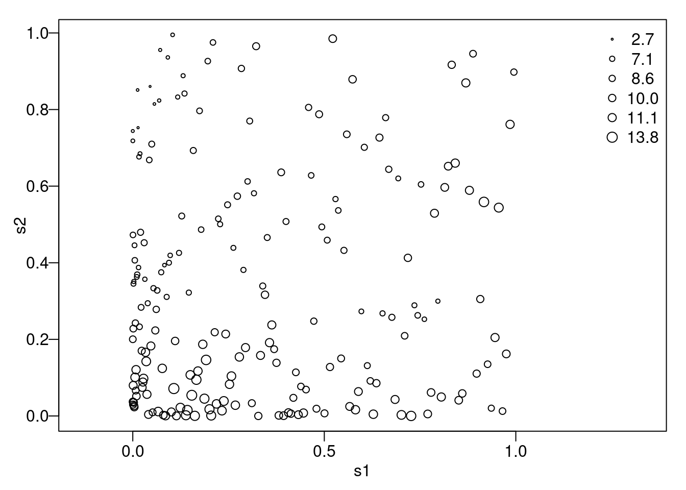
Figure 2.3: The simulated toy example data.
These data will be used as a toy example in this tutorial. It is available in
the R-INLA package and can be loaded by typing:
data(SPDEtoy)2.2 The SPDE approach
Rue and Tjelmeland (2002) propose to approximate a continuous Gaussian field using
GMRFs, and demonstrated good fits for a range of commonly used
covariance functions. Although these “proof-of-concept” results were
interesting, their approach was less practical. All fits had to be
precomputed on a regular grid only. The real breakthrough, came with
Lindgren, Rue, and Lindström (2011), who considered a stochastic partial differential
equation (SPDE) whose solution is a GF with Matérn correlation.
Lindgren, Rue, and Lindström (2011) propose a new approach to represent a GF with Matérn
covariance, as a GMRF, by representing a solution of the SPDE using
the finite element method. This was possible only for some values of
the smoothness \(\nu\), where the continuous indexed random field was
Markov (Rozanov (1977)). The benefit is that the GMRF representation of
the GF, which can be computed explicitly, provides a sparse
representation of the spatial effect through a sparse precision
matrix. This enables the nice computational properties of the GMRFs
which can then be implemented in the INLA package.
Warning. In this section the main results in Lindgren, Rue, and Lindström (2011) are
summarized. If your purpose does not include understanding the
underlying methodology in depth, you can skip this section. If you
keep reading this section and find it difficult, do not be
discouraged. You will still be able to use INLA for applications even if
you have only a limited grasp of what is “under the hood”.
In this section we have tried to provide an intuitive approach to SPDE. However, if you are interested in the full details, they are in the Appendix of Lindgren, Rue, and Lindström (2011). In a few words, it uses the Finite Element Method (FEM, Ciarlet 1978; Brenner and Scott 2007; Quarteroni and Valli 2008) to provide a solution to a SPDE. They develop this solution by considering basis functions carefully chosen to preserve the sparse structure of the resulting precision matrix for the random field at a set of mesh nodes. This provides an explicit link between a continuous random field and a GMRF representation, which allows efficient computations.
2.2.1 First result
The first main result provided in Lindgren, Rue, and Lindström (2011) is that a GF with a generalized covariance function, obtained when \(\nu > 0\) in the Matérn correlation function is a solution to a SPDE. This extends the result obtained by Besag (1981). A more statistical way to look at this result is by considering a regular two-dimensional lattice with number of sites tending to infinity. The representation of sites in a lattice can be seen in Figure 2.4.
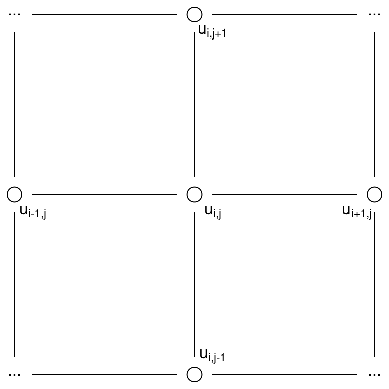
Figure 2.4: Representation of sites in a two-dimensional lattice to estimate a spatial process.
In this case the full conditional distribution at the site \(i,j\) has expectation
\[ E(u_{i,j}|u_{-i,j}) = \frac{1}{a}(u_{i-1,j}+u_{i+1,j}+u_{i,j-1}+u_{i,j+1}) \]
and variance \(Var(u_{i,j}|u_{-i,j}) = 1/a\), with \(|a|>4\). In the representation using a precision matrix, for a single site, only the upper right quadrant is shown and with \(a\) as the central element, such that
\[\begin{equation} \tag{2.4} \begin{array}{|cc} -1 & \\ a & -1 \\ \hline \end{array} \end{equation}\]
A GF \(U(\mathbf{s})\) with Matérn covariance is a solution to the following linear fractional SPDE:
\[ (\kappa^2 - \Delta )^{\alpha/2}u(\mathbf{s}) = \mathbf{W}(\mathbf{s}),\;\;\; \mathbf{s} \in \mathbb{R}^d,\;\;\;\alpha=\nu+d/2,\;\;\kappa>0,\;\;\nu>0. \]
Here, \(\Delta\) is the Laplacian operator and \(\mathbf{W}(\mathbf{s})\) denotes a spatial white noise Gaussian stochastic process with unit variance.
Lindgren, Rue, and Lindström (2011) show that, for \(\nu=1\) and \(\nu=2\), the GMRF representation is a convolution of processes with precision matrix as in Equation (2.4). The resulting upper right quadrant precision matrix and center can be expressed as a convolution of the coefficients in Equation (2.4). For \(\nu=1\), using this representation, we have:
\[\begin{equation} \tag{2.5} \begin{array}{|ccc} 1 & & \\ -2a & 2 & \\ 4+a^2 & -2a & 1 \\ \hline \end{array} \end{equation}\]
and, for \(\nu=2\):
\[\begin{equation} \tag{2.6} \begin{array}{|cccc} -1 & & & \\ 3a & -3 & & \\ -3(a^2+3) & 6a & -3 & \\ a(a^2+12) & -3(a^2+3) & 3a & -1 \\ \hline \end{array} \end{equation}\]
An intuitive interpretation of this result is that as the smoothness parameter \(\nu\) increases, the precision matrix in the GMRF representation becomes less sparse. Greater density of the matrix is due to the fact that the conditional distributions depend on a wider neighborhood. Notice that it does not imply that the conditional mean is an average over a wider neighborhood.
Conceptually, this is like going from a first order random walk to a second order one. To understand this point, let us consider the precision matrix for the first order random walk, its square, and the precision matrix for the second order random walk.
q1 <- INLA:::inla.rw1(n = 5)
q1
## 5 x 5 sparse Matrix of class "dgTMatrix"
##
## [1,]  1 -1  .  .  .
## [2,] -1  2 -1  .  .
## [3,]  . -1  2 -1  .
## [4,]  .  . -1  2 -1
## [5,]  .  .  . -1  1
# Same inner pattern as for RW2
crossprod(q1)
## 5 x 5 sparse Matrix of class "dsCMatrix"
##
## [1,]  2 -3  1  .  .
## [2,] -3  6 -4  1  .
## [3,]  1 -4  6 -4  1
## [4,]  .  1 -4  6 -3
## [5,]  .  .  1 -3  2
INLA:::inla.rw2(n = 5)
## 5 x 5 sparse Matrix of class "dgTMatrix"
##
## [1,]  1 -2  1  .  .
## [2,] -2  5 -4  1  .
## [3,]  1 -4  6 -4  1
## [4,]  .  1 -4  5 -2
## [5,]  .  .  1 -2  1
As can be seen in the previous matrices, the differences between the precision matrix of a random walk of order 2 and the crossproduct of a precision matrix of a random walk of order 1 appear at the upper-left and bottom-right corners. The precision matrix for \(\alpha=2\), \(\mathbf{Q}_2=\mathbf{Q}_1\mathbf{C}^{-1}\mathbf{Q}_1\), is a standardized square of the precision matrix for \(\alpha=1\), \(\mathbf{Q}_1\). Matrices \(\mathbf{Q}_1\), \(\mathbf{C}\) and \(\mathbf{Q}_2\) are fully described later in Section 2.2.2.
2.2.2 Second result
Point data are seldom located on a regular grid but distributed irregularly. Lindgren, Rue, and Lindström (2011) provide a second set of results that give a solution for the case of irregular grids. This was made considering the FEM, which is widely used in engineering and applied mathematics to solve differential equations.
The domain can be divided into a set of non-intersecting triangles, which may be irregular, where any two triangles meet in at most a common edge or corner. The three corners of a triangle are named vertices or nodes. The solution for the SPDE and its properties will depend on the basis functions used. Lindgren, Rue, and Lindström (2011) choose basis functions carefully in order to preserve the sparse structure of the resulting precision matrix.
The approximation is:
\[\begin{equation} \tag{2.7} u(\mathbf{s}) = \sum_{k=1}^{m}\psi_k(\mathbf{s})w_k \end{equation}\]
where \(\psi_k\) are basis functions and \(w_k\) are Gaussian distributed weights,
\(k=1,...,m\), with \(m\) the number of vertices in the triangulation. A
stochastic weak solution was considered to show that the joint distribution for
the weights determines the full distribution in the continuous domain.
More information about the weak solution and how to use the FEM in this case can be found in Bakka (2018).
We will now illustrate how the process \(u(\mathbf{s})\) can be approximated to any point inside the triangulated domain. First, we consider the one-dimensional case in Figure 2.5. We have a set of six piece-wise linear basis functions shown at the top of this figure. The value of each of such basis functions is one at the basis knot, decreases linearly to zero until the center of the next basis function and is zero elsewhere. Thus for any point between two basis knots only two basis functions have a non-zero value. At the bottom of Figure 2.5, we have the sine function that was approximated using these basis functions. Note that we have used irregularly spaced knots here. Thus, the intervals between the knots do not need to be equally spaced (in a similar way as triangles in a mesh do not need to be equal). For example, it will be better to place more knots (or triangles in space) where the function changes more rapidly, as we did considering a knot at 1.5, shown in Figure 2.5. From this figure it is also clear that it would be better to have one knot around 4.5 as well.
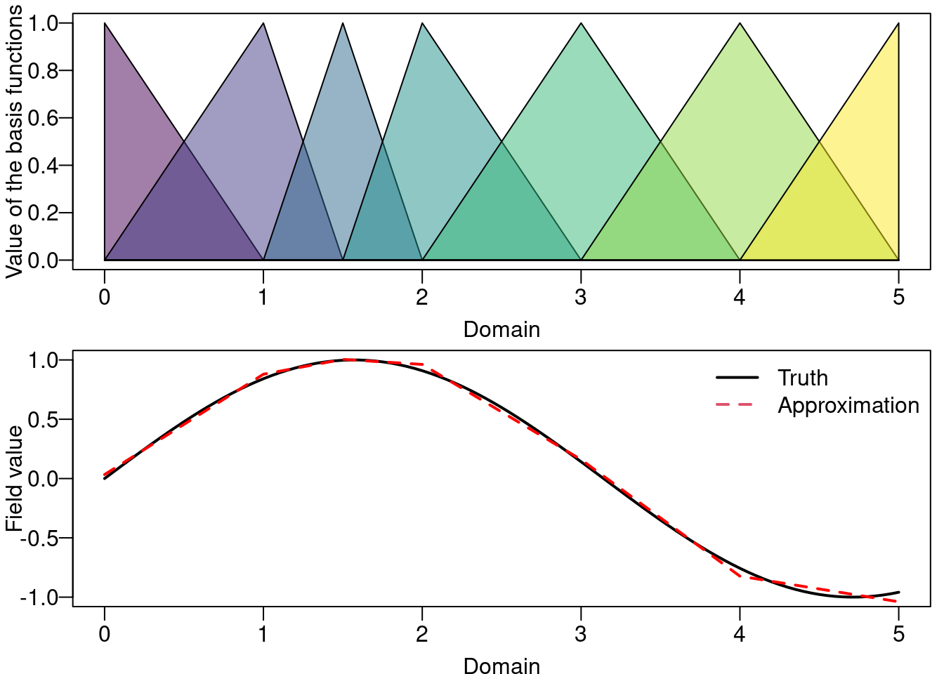
Figure 2.5: One dimensional approximation illustration. The one dimensional piece-wise linear basis functions (top). A function and its approximation (bottom).
We now illustrate the approximation in two dimensional space considering piece-wise linear basis functions. These are based on triangles as a generalization of the idea in one dimension. Consider the big triangle shown on the top left of Figure 2.6, the point shown as a red dot inside this big triangle, and the three small triangles formed by this point and each vertex of the big one. The numbers at the vertex of the big triangle are equal to the area of the opposite triangle inside the big one (not formed by this vertex), divided by the area total of the big triangle. Thus, the three numbers sum up to one. These three numbers are the value of the basis function centered at the vertices of the big triangle being evaluated at the red point. These three values are considered for the approximation as they are the coefficients that multiply the function at each vertex of the big triangle.
Writing in matrix form, we have the projector matrix \(\mathbf{A}\) and when a point is inside a triangle, there are three non-zero values in the corresponding line of \(\mathbf{A}\). When the point is along an edge, there are two non-zero values and when the point is on top of a triangle vertex there is only one non-zero (which is equal to one). This is just an illustration of the barycentric coordinates of the point with respect to the coordinates of the triangle vertices known also as areal coordinates for this particular case.
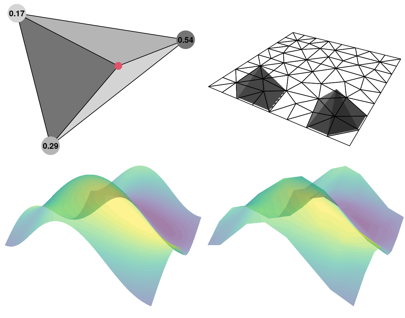
Figure 2.6: Two dimensional approximation illustration. A triangle and the areal coordinates for the point in red (top left). All the triangles and the basis function for two of them (top right). A true field for illustration (bottom left) and its approximated version (bottom right).
We will now focus on the resulting precision matrix of the observations \(\mathbf{Q}_{\alpha,\kappa}\). It does consider the triangulation and the basis functions. The precision matrix matches the first result when applied to a regular grid. Consider the set of \(m\times m\) matrices \(\mathbf{C}\), \(\mathbf{G}\) and \(\mathbf{K}_{\kappa}\) with entries
\[ \mathbf{C}_{i,j} = \langle \psi_i, \psi_j\rangle, \;\;\;\;\; \mathbf{G}_{i,j} = \langle \nabla \psi_i, \nabla \psi_j \rangle, \;\;\;\;\; (\mathbf{K}_{\kappa})_{i,j} = \kappa^2 C_{i,j} + G_{i,j}\;. \]
Here, \(\langle \cdot, \cdot \rangle\) denotes the inner product and \(\nabla\) the gradient.
The precision matrix \(\mathbf{Q}_{\alpha,\kappa}\) as a function of \(\kappa^2\) and \(\alpha\) can be written as:
\[\begin{equation} \tag{2.8} \begin{array}{rcl} \mathbf{Q}_{1,\kappa} & = & \mathbf{K}_{\kappa} = \kappa^2\mathbf{C} + \mathbf{G}, \\ \mathbf{Q}_{2,\kappa} & = & \mathbf{K}_{\kappa}\mathbf{C}^{-1}\mathbf{K}_{\kappa} = \kappa^4\mathbf{C} + 2\kappa^2\mathbf{G} + \mathbf{G}\mathbf{C}^{-1}\mathbf{G} \\ \mathbf{Q}_{\alpha,\kappa} & = & \mathbf{K}_{\kappa}\mathbf{C}^{-1}Q_{\alpha-2,\kappa}\mathbf{C}^{-1}\mathbf{K}_{\kappa}, \;\;\;\mbox{for} \;\;\alpha = 3,4,...\;. \end{array} \end{equation}\]
Matrices \(\mathbf{C}\) and \(\mathbf{C}^{-1}\) can be replaced by \(\tilde{\mathbf{C}}\) and \(\tilde{\mathbf{C}}^{-1}\), respectively, with \(\tilde{\mathbf{C}}\) a diagonal matrix with diagonal elements
\[\begin{align} \tilde{\mathbf{C}}_{i,i} = \langle \psi_i, 1 \rangle, \end{align}\]
which is common when working with FEM. In this case, since \(\tilde{\mathbf{C}}\) is diagonal, \(\mathbf{K}_{\kappa}\) is as sparse as \(\mathbf{G}\).
As an example, we consider a set of seven points and build a mesh around four of them with an adequate choice of the arguments in order to have a didactic illustration of the FEM. The dual mesh is also built. Finally, the code extracts matrices \(\mathbf{C}\), \(\mathbf{G}\) and \(\mathbf{A}\):
# This 's' factor will only change C, not G
s <- 3
pts <- cbind(c(0.1, 0.9, 1.5, 2, 2.3, 2, 1),
  c(1, 1, 0, 0, 1.2, 1.9, 2)) * s
n <- nrow(pts)
mesh <- inla.mesh.2d(pts[-c(3, 5, 7), ], max.edge = s * 1.7,
  offset = s / 4, cutoff = s / 2, n = 6)
m <- mesh$n
dmesh <- book.mesh.dual(mesh)
fem <- inla.mesh.fem(mesh, order = 1)
A <- inla.spde.make.A(mesh, pts)
Here, function book.mesh.dual() is used to create the dual mesh polygons
(see Figure 2.7). Furthermore, function inla.mesh.fem() is
used to create matrices \(\mathbf{C}\) and \(\mathbf{G}\), while function
inla.spde.make.A() creates the projector matrix \(\mathbf{A}\).
We can gain intuition about this result by considering the structure of each matrix, which is detailed in Appendix A.2 in Lindgren, Rue, and Lindström (2011). It may be easier to understand it by considering the plots in Figure 2.7. In this figure, a mesh with 8 nodes is shown in thicker border lines. The corresponding dual mesh forms a collection of polygons around each vertex of the mesh.
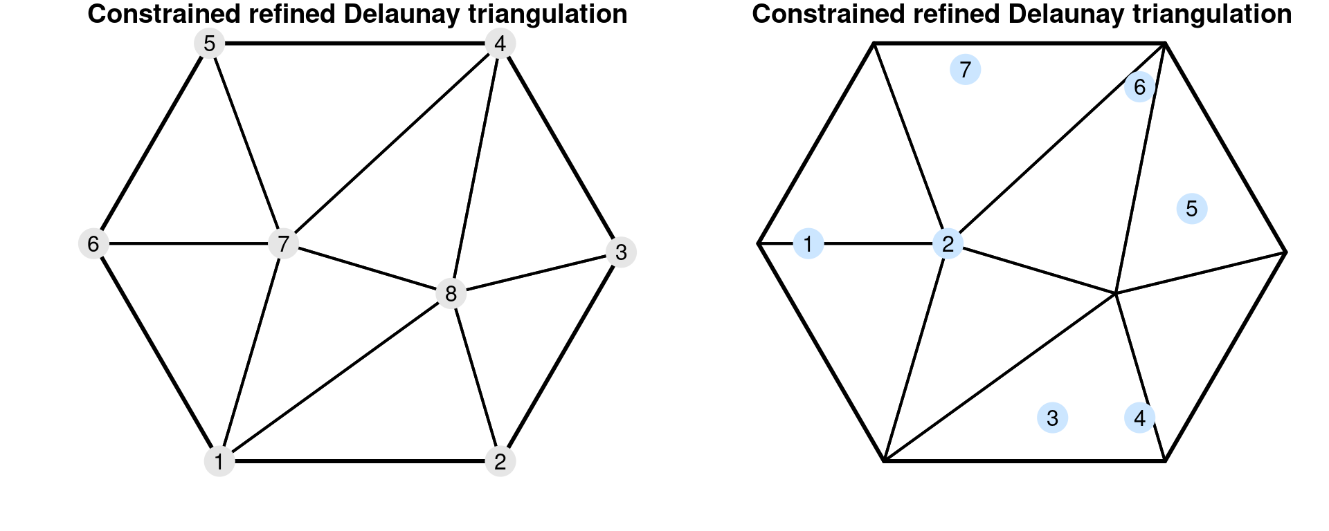
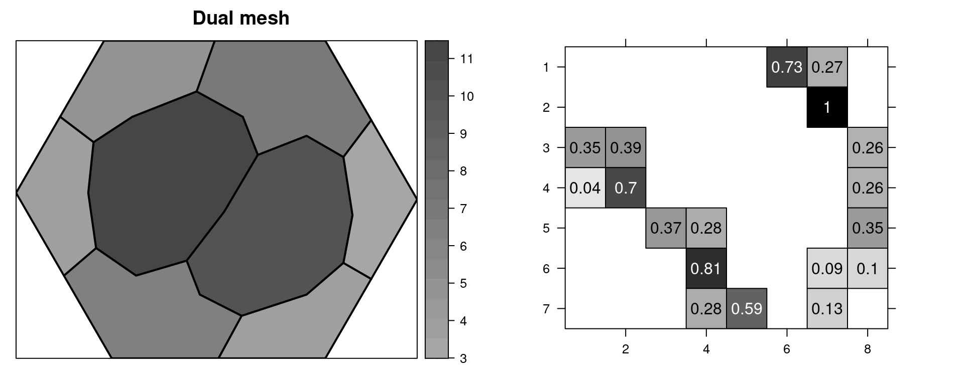
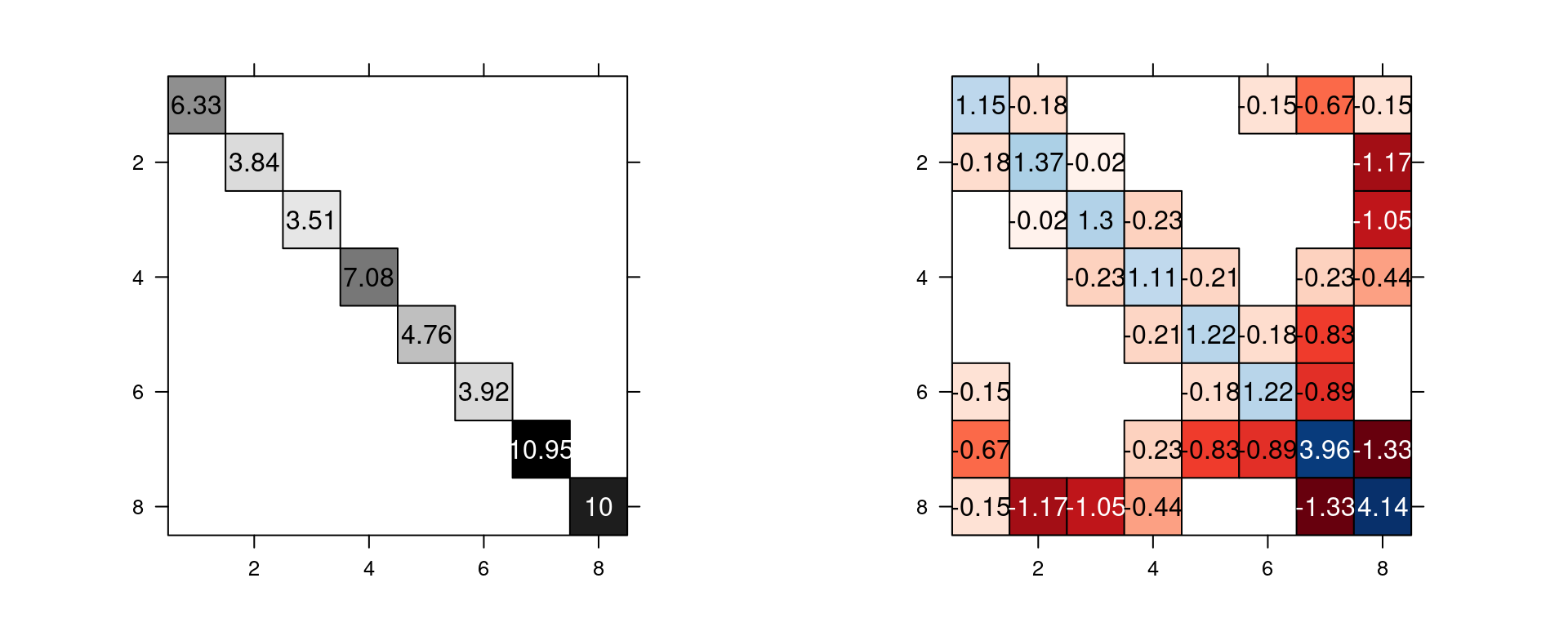
Figure 2.7: A mesh and its nodes numbered (top left) and the mesh with some points numbered (top right). The dual mesh polygons (mid left) and \(\mathbf{A}\) matrix (mid right). The associated \(\mathbf{C}\) matrix (bottom left) and \(\mathbf{G}\) matrix (bottom center).
The dual mesh is a set of polygons, one polygon for each vertex. Each polygon is formed by the mid of each of the edges that connects to the vertex, and the centroids of the triangles that the vertex is a corner of. Notice that for the vertices at the boundary of the mesh, this vertex is one point of the dual polygon as well. The area of each dual polygon is equal to \(\tilde{\mathbf{C}}_{ii}\).
Equivalently, \(\tilde{\mathbf{C}}_{ii}\) is equal to the sum of one third the area of each triangle that the vertex \(i\) is part of. Notice that each polygon around each mesh node is formed by one third of the triangles that it is part of. The \(\tilde{\mathbf{C}}\) matrix is diagonal.
Matrix \(\mathbf{G}\) reflects the connectivity of the mesh nodes. Nodes not connected by edges have the corresponding entry as zero. Values do not depend on the size of the triangles as they are scaled by the area of the triangles. For more detailed information, see Appendix 2 in Lindgren, Rue, and Lindström (2011).
As stated above, the resulting precision matrix for increasing \(\nu\) is a convolution of the precision matrix for \(\nu-1\) with a scaled \(\mathbf{K}_{\kappa}\). It still implies a denser precision matrix when working with \(\kappa\mathbf{C} + \mathbf{G}\).
The \(\mathbf{Q}\) precision matrix can be generalized to fractional values of \(\alpha\) (or \(\nu\)) using a Taylor approximation. See the author’s discussion response in Lindgren, Rue, and Lindström (2011). This approximation leads to a polynomial of order \(p = \lceil \alpha \rceil\) for the precision matrix:
\[\begin{equation} \tag{2.9} \mathbf{Q} = \sum_{i=0}^p b_i \mathbf{C}(\mathbf{C}^{-1}\mathbf{G})^i. \end{equation}\]
For \(\alpha=1\) and \(\alpha=2\), the precision matrix is the same as in Equation (2.8). For \(\alpha=1\), the values of the coefficients of the Taylor approximation are \(b_0=\kappa^2\) and \(b_1=1\). For the case \(\alpha=2\), the coefficients are \(b_0=\kappa^4\), \(b_1=\alpha\kappa^4\) and \(b_2=1\).
For fractional \(\alpha=1/2\), it holds that \(b_0=3\kappa/4\) and \(b_1=\kappa^{-1}3/8\). And for \(\alpha=3/2\) (and \(\nu=0.5\), the exponential case), the values are \(b_0=15\kappa^3/16\), \(b_1=15\kappa/8\) and \(b_2=15\kappa^{-1}/128\). Using these results combined with a recursive construction, for \(\alpha>2\), GMRF approximations can be obtained for all positive integers and half-integers.
2.3 A toy example
In this example we will fit a simple geostatistical model to the toy dataset
simulated in Section 2.1.4. This dataset is also available in the
INLA package and it can be loaded as follows:
data(SPDEtoy)This dataset is a three-column data.frame. Coordinates are in the first
two columns and the response in the third column.
str(SPDEtoy)
## 'data.frame':    200 obs. of  3 variables:
##  $ s1: num  0.0827 0.6123 0.162 0.7526 0.851 ...
##  $ s2: num  0.0564 0.9168 0.357 0.2576 0.1541 ...
##  $ y : num  11.52 5.28 6.9 13.18 14.6 ...
2.3.1 SPDE model definition
Given \(n\) observations \(y_i\), \(i=1,...,n\), at locations \(\mathbf{s}_i\), the following model can be defined:
\[ \begin{array}{rcl} \mathbf{y}|\beta_0,\mathbf{u},\sigma_e^2 & \sim & N(\beta_0 + \mathbf{A} \mathbf{u}, \sigma_e^2) \\ \mathbf{u} & \sim & GF(0, \Sigma) \end{array} \]
where \(\beta_0\) is the intercept, \(\mathbf{A}\) is the projector matrix and \(\mathbf{u}\) is a spatial Gaussian random field. Note that the projector matrix \(\mathbf{A}\) links the spatial Gaussian random field (defined using the mesh nodes) to the locations of the observed data.
This mesh must cover the entire spatial domain of interest. More details on
mesh building are given in Section 2.6. Here, the
fifth mesh built in Section 2.6.3 will be used. In the
following R code, a domain is first defined to create the mesh:
pl.dom <- cbind(c(0, 1, 1, 0.7, 0), c(0, 0, 0.7, 1, 1))
mesh5 <- inla.mesh.2d(loc.domain = pl.dom, max.e = c(0.092, 0.2))
The SPDE model in the original parameterization can be built
using function inla.spde2.matern().
The main arguments of this function
are the mesh object (mesh) and the \(\alpha\) parameter
(alpha), which is related to the smoothness parameter of the process. The
parameterization is flexible and can be defined by the user, with a default
choice controlling the log of \(\tau\) and \(\kappa\), that jointly control the
variance and correlation range.
Instead of using the default parameterization, it is more intuitive to control
the parameters through the marginal standard deviation and the range,
\(\sqrt{8\nu}/\kappa\). For details on this parameterization see Lindgren (2012).
In addition, when defining the SPDE model a set of priors for both parameters is
also required. The inla.spde2.pcmatern() uses this parameterization to set
the Penalized Complexity prior, PC-prior, as derived in Fuglstad et al. (2018).
The Penalized Complexity prior is under the framework reviewed in Section
1.6.5.
The PC-prior was derived for the practical range, or just range,
which is the distance such that the correlation is around \(0.139\),
and the marginal standard deviation of the field, \(\sigma\).
The way of setting these priors for \(\sigma\) is that we do need to
set \(\sigma_0\) and \(p\) such that P\((\sigma>\sigma_0)=p\).
In our example we will set \(\sigma_0=10\) and \(p=0.01\) and
these values are passed to the inla.spde2.matern() function
as a vector in the next code.
For the practical range parameter the setting is that we have to
choose \(r_0\) and \(p\) such that P\((r<r_0)=p\).
We have to account for the fact that in our example the domain
is the \([0,1]\times [0,1]\) square.
We can set the PC-prior for the median by setting \(p=0.5\)
and in the next code we consider a prior median equal to \(0.3\).
The smoothness parameter \(\nu\) is fixed as \(\alpha=\nu+d/2\in [1,2]\).
Next, we build the SPDE model considering that the toy data was simulated
with \(\alpha=2\), which is actually the default value in the
inla.spde2.pcmatern() function:
spde5 <- inla.spde2.pcmatern(
  # Mesh and smoothness parameter
  mesh = mesh5, alpha = 2,
  # P(practic.range < 0.3) = 0.5
  prior.range = c(0.3, 0.5),
  # P(sigma > 1) = 0.01
  prior.sigma = c(10, 0.01))
2.3.2 Projector matrix
The second step when setting an SPDE model is to build a projector matrix. The
projector matrix contains the basis function value for each basis, with one
basis function at each column. It will be used to interpolate the random field
that is being modeled at the mesh nodes. For details, see Section
2.2.2. The projector matrix can be built with the
inla.spde.make.A() function. Considering the basis function at each mesh
vertex, the basis function value for one point within one triangle is computed
as illustrated in Figure 2.6. Thus, the value for the random
field is the projection of a plane (formed by the random field value at these
three mesh points) to this point location. This is why we call a projector matrix
to the matrix that stores in each line a different basis function evaluated at
a location point. This matrix is sparse since no more than three elements in
each line are non-zero. Also, the sum of each row is equal to one.
Using the toy dataset and example mesh mesh5, the projector matrix can be
computed as follows:
coords <- as.matrix(SPDEtoy[, 1:2])
A5 <- inla.spde.make.A(mesh5, loc = coords)
This matrix has dimension equal to the number of data locations times the number of vertices in the mesh:
dim(A5)
## [1] 200 490
Because each point location is inside one of the triangles there are exactly three non-zero elements on each line:
table(rowSums(A5 > 0))
##
##   3
## 200
Furthermore, these three elements on each line sum up to one:
table(rowSums(A5))
##
##   1
## 200
The reason why they sum up to one is that each matrix element is a basis function evaluated at a point location, and the basis functions sum up to one at each location. Multiplication of this matrix by a vector representing a continuous function evaluated at the locations gives the interpolation of this function at the point locations.
There are some columns in the projector matrix all of whose elements equal zero:
table(colSums(A5) > 0)
##
## FALSE  TRUE
##   242   248
These columns correspond to triangles with no point location inside. These
columns can be dropped. The inla.stack() function (Section 2.3.3)
does this automatically.
When there is a mesh where every point location is at a mesh vertex, each line
on the projector matrix has exactly one non-zero element. This is the case for
the mesh1 built in Section 2.6.3:
A1 <- inla.spde.make.A(mesh1, loc = coords)In this case, all the non-zero elements in the projector matrix are equal to one:
table(as.numeric(A1))
##
##      0      1
## 579800    200
Each element is equal to one in this case because the location points are actually one of the mesh nodes and thus the weight of the basis function at one mesh node is equal to one.
2.3.3 The data stack
The inla.stack() function is useful for organizing data, covariates, indices
and projector matrices, all of which are important when constructing an SPDE
model. inla.stack() helps to control the way effects are projected in the
linear predictor. Detailed examples including one dimensional, replicated
random field and space-time models are presented in Lindgren (2012) and
Lindgren and Rue (2015), which also details the mathematical theory for the stack
method.
In the toy example, there is a linear predictor that can be written as
\[ \mathbf{\eta}^{*} = \mathbf{1}\beta_0 + \mathbf{A}\mathbf{u} \;. \]
The first term on the right-hand side represents the intercept, while the second represents the spatial effect. Each term is represented as a product of a projector matrix and an effect.
The solution obtained with the Finite Element Method considered when
implementing the SPDE models builds the model on the mesh nodes. Usually, the
number of nodes is not equal to the number of locations for which we have
observations. The inla.stack() function allows us to work with predictors
that includes terms with different dimensions. The three main inla.stack()
arguments are a vector list with the data (data), a list of projector
matrices (each related to one block effect, A) and the list of effects
(effects). Optionally, a label can be assigned to the data stack (using
argument tag).
Two projector matrices are needed: the projector matrix for the latent field and a matrix that is a one-to-one map of the covariate and the response. The latter matrix can simply be a constant rather than a diagonal matrix.
The following R code will take the toy example data and use function
inla.stack() to put all these three elements (i.e., data, projector matrices
and effects) together:
stk5 <- inla.stack(
  data = list(resp = SPDEtoy$y),
  A = list(A5, 1),
  effects = list(i = 1:spde5$n.spde,
    beta0 = rep(1, nrow(SPDEtoy))),
  tag = 'est')
The inla.stack() function automatically eliminates any column in a projector
matrix that has a zero sum, and it generates a new and simplified matrix. The
function inla.stack.A() extracts a simplified matrix to use as an observation
predictor matrix with the inla() function, while the inla.stack.data()
function extracts the corresponding data.
The simplified projector matrix from the stack consists of the simplified projector matrices, where each column holds one effect block. Hence, its dimensions are:
dim(inla.stack.A(stk5))
## [1] 200 249
In the toy example, there is one column more than the number of columns with non-zero elements in the projector matrix. This extra column is due to the intercept and all values are equal to one.
2.3.4 Model fitting and some results
To fit the model, the intercept in the formula must be removed and added as a
covariate term in the list of effects, so that all the covariate terms in the
formula can be included in a projector matrix. Then, the matrix of predictors
is passed to the inla() function in its control.predictor
argument, as follows:
res5 <- inla(resp ~ 0 + beta0 + f(i, model = spde5),
  data = inla.stack.data(stk5),
  control.predictor = list(A = inla.stack.A(stk5)))
The inla() function returns an object that is a set of several results. It
includes summaries, marginal posterior densities of each parameter in the
model, the regression parameters, each element that is a latent field, and all
the hyperparameters.
The summary of the intercept \(\beta_0\) is obtained with the following R code:
res5$summary.fixed
##        mean     sd 0.025quant 0.5quant 0.975quant  mode
## beta0 9.525 0.6932      8.073    9.539      10.89 9.559
##             kld
## beta0 6.141e-10
Similarly, the summary of the precision of the Gaussian likelihood, i.e., \(1/\sigma_e^2\), can be obtained as follows:
res5$summary.hyperpar[1, ]
##                                          mean     sd
## Precision for the Gaussian observations 2.744 0.4268
##                                         0.025quant 0.5quant
## Precision for the Gaussian observations      1.997    2.713
##                                         0.975quant  mode
## Precision for the Gaussian observations      3.673 2.654
A marginal distribution in the inla() output consists of two vectors. One is
a set of values on the range of the parameter space with posterior marginal
density bigger than zero and another is the posterior marginal density at each
one of these values. Any posterior marginal can be transformed. For example,
if the posterior marginal for \(\sigma_e\) is required, the square root of \(\sigma_e^2\),
it can be obtained as follows:
post.se <- inla.tmarginal(function(x) sqrt(1 / exp(x)),
  res5$internal.marginals.hyperpar[[1]])
Now, it is possible to obtain summary statistics from this marginal distribution:
inla.emarginal(function(x) x, post.se)
## [1] 0.6091
inla.qmarginal(c(0.025, 0.5, 0.975), post.se)
## [1] 0.5224 0.6070 0.7067
inla.hpdmarginal(0.95, post.se)
##               low   high
## level:0.95 0.5189 0.7026
inla.pmarginal(c(0.5, 0.7), post.se)
## [1] 0.005309 0.966850
In the previous code, function inla.emarginal() is used to compute the
posterior expectation of a function on the parameter, function
inla.qmarginal() computes quantiles from the posterior marginal, function
inla.hpdmarginal() computes a highest posterior density (HPD) interval and
function inla.pmarginal() can be used to obtain posterior probabilities.
Figure 2.8 shows the posterior marginals of the precision and the
standard deviation, which has been created with the following code:
par(mfrow = c(1, 2), mar = c(3, 3, 1, 1), mgp = c(2, 1, 0))
plot(res5$marginals.hyperpar[[1]], type = "l", xlab = "precision",
     ylab = "density", main = "Precision")
plot(post.se, type = "l", xlab = "st. deviation",
     ylab = "density", main = "Standard deviation")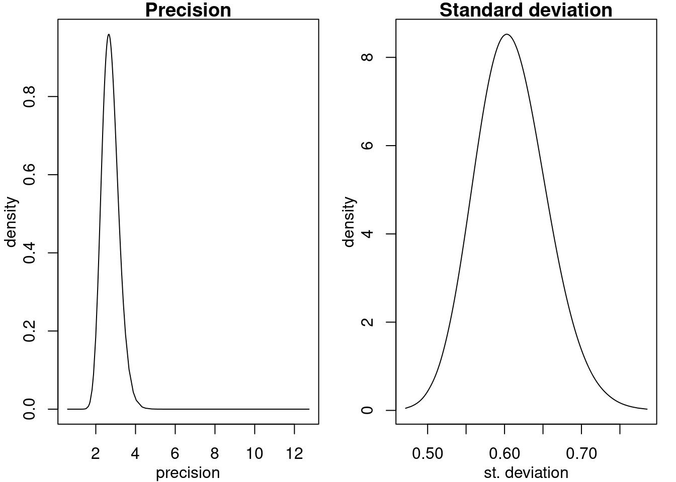
Figure 2.8: Posterior marginals of the precision (top) and the standard deviation (bottom).
In cases with weakly identifiable parameters, transforming the posterior marginal densities leads to a loss of accuracy. To reduce that loss, one can operate more directly on the marginal densities without first transforming:
post.orig <- res5$marginals.hyperpar[[1]]
fun <- function(x) rev(sqrt(1 / x)) # Use rev() to preserve order
ifun <- function(x) rev(1 / x^2)
inla.emarginal(fun, post.orig)
## [1] 0.5466
fun(inla.qmarginal(c(0.025, 0.5, 0.975), post.orig))
## [1] 0.5223 0.6072 0.7074
fun(inla.hpdmarginal(0.95, post.orig))
## [1] 0.5274 0.7169
inla.pmarginal(ifun(c(0.5, 0.7)), post.orig)
## [1] 0.03403 0.99427
Note that the HPD interval is not invariant to changes of variables, and if a specific interpretation is required one therefore has to start by transforming the density to that parameterization.
The posterior marginals for the parameters of the latent field are visualized in Figure 2.9 with:
par(mfrow = c(2, 1), mar = c(3, 3, 1, 1), mgp = c(2, 1, 0))
plot(res5$marginals.hyperpar[[2]], type = "l",
  xlab = expression(sigma), ylab = 'Posterior density')
plot(res5$marginals.hyperpar[[3]], type = "l",
  xlab = 'Practical range', ylab = 'Posterior density')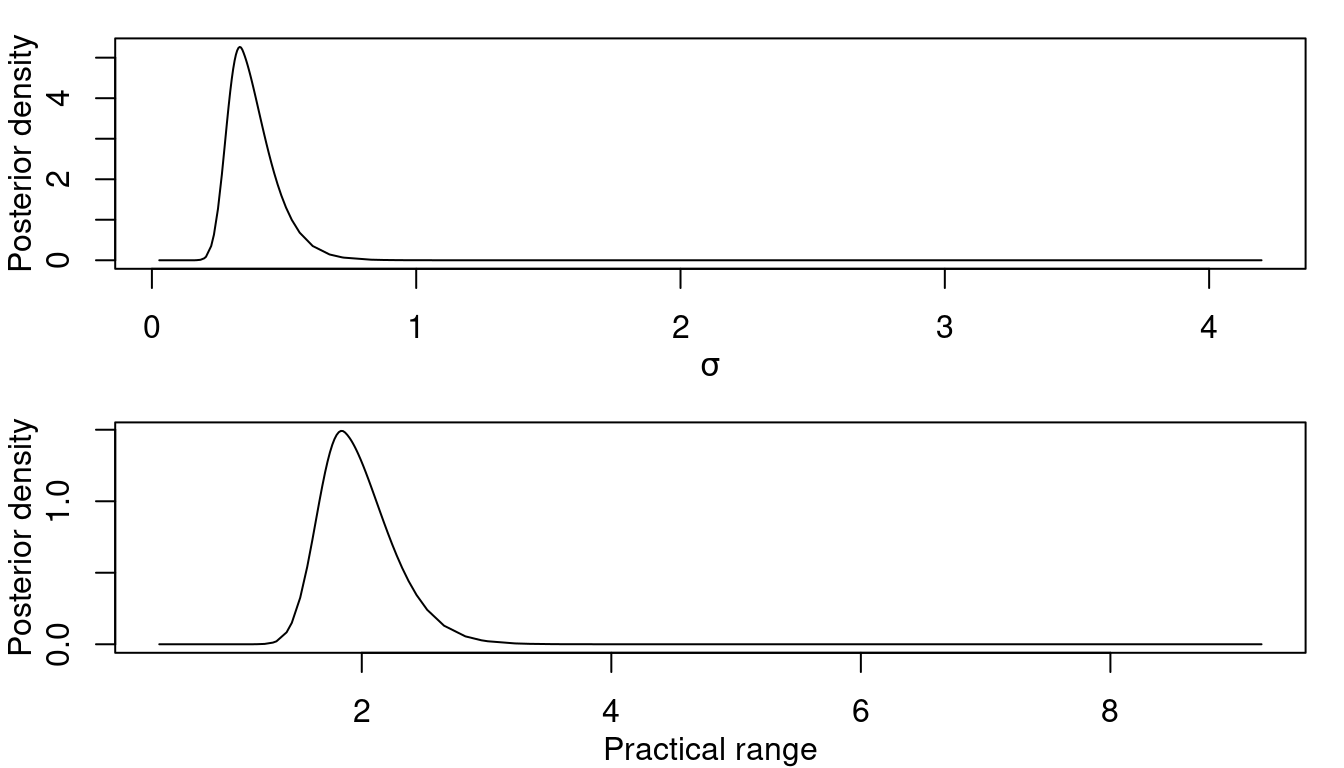
Figure 2.9: Posterior marginal distribution for \(\sigma\) (left) and the practical range (right).
Furthermore, summary statistics and HPD intervals can also be computed, and these marginals can be plotted as well to visualize them.
2.4 Projection of the random field
A common objective when dealing with spatial data collected at some locations is the prediction on a fine grid of the spatial model to get high resolution maps. In this section we show how to do this prediction for the random field term only. In Section 2.5, prediction of the outcome will be described. In this example, the random field will be predicted at three target locations: (0.1, 0.1), (0.5, 0.55), (0.7, 0.9). These points are defined in the following code:
pts3 <- rbind(c(0.1, 0.1), c(0.5, 0.55), c(0.7, 0.9))The predictor matrix for the target locations is:
A5pts3 <- inla.spde.make.A(mesh5, loc = pts3)
dim(A5pts3)
## [1]   3 490
In order to visualize only the columns with non-zero elements of this matrix, the following code can be run:
jj3 <- which(colSums(A5pts3) > 0)
A5pts3[, jj3]
## 3 x 9 sparse Matrix of class "dgCMatrix"
##
## [1,] .    .    0.094 .    .    .    0.51 0.39 .
## [2,] 0.22 .    .     0.32 .    0.46 .    .    .
## [3,] .    0.12 .     .    0.27 .    .    .    0.61
This projector matrix can then be used for interpolating a functional of the random field, for example, the posterior mean. This interpolation is a computationally very cheap operation, since it is a matrix vector product where the matrix is sparse, having only up to three non-zero elements in each row.
drop(A5pts3 %*% res5$summary.random$i$mean)
## [1]  0.1489  3.0358 -2.7686
2.4.1 Projection on a grid
By default, the inla.mesh.projector() function computes a projector matrix
automatically for a grid of points over a square that contains the mesh. It
can be used to get the map of the random field on a fine grid. To get a
projector matrix on a grid in the domain \([0, 1]\times [0, 1]\) these limits can
be passed to the inla.mesh.projector() function:
pgrid0 <- inla.mesh.projector(mesh5, xlim = 0:1, ylim = 0:1,
  dims = c(101, 101))
Then, the projection of the posterior mean and the posterior standard deviation can be obtained with the following code:
prd0.m <- inla.mesh.project(pgrid0,  res5$summary.random$i$mean)
prd0.s <- inla.mesh.project(pgrid0,  res5$summary.random$i$sd)
The values projected on the grid are available in Figure 2.10.
2.5 Prediction
Another quantity of interest when modeling spatially continuous processes is the prediction of the expected value on a target location for which data have not been observed. In a similar way as in the previous section, it is possible to compute the marginal distribution of the expected value at the target location or to make a projection of some functional of it, specifically, considering that
\[ \mathbf{y} \sim N(\mathbf{\mu} = \mathbf{1}\beta_0 + \mathbf{A} \mathbf{u}, \sigma_e^2\mathbf{I}). \]
We will be computing the posterior distribution of \(\mathbf{\mu}\). This problem is often called prediction.
2.5.1 Joint estimation and prediction
In this case, we just set a scenario for the prediction and include it in the stack used in the model fitting. This is similar to the stack created to predict the random field, but here all the fixed effects have to be considered in the predictor and effects slots of the stack. In our case we just have the intercept:
stk5.pmu <- inla.stack(
  data = list(resp = NA),
  A = list(A5pts3, 1),
  effects = list(i = 1:spde5$n.spde, beta0 = rep(1, 3)),
  tag = 'prd5.mu')
This stack is then joined to the data stack to fit the model again. Notice we
can save time by considering the previous fitted model parameters here (by
using parameter control.mode):
stk5.full <- inla.stack(stk5, stk5.pmu)
r5pmu <- inla(resp ~ 0 + beta0 + f(i, model = spde5),
  data = inla.stack.data(stk5.full),
  control.mode = list(theta = res5$mode$theta, restart = FALSE),
  control.predictor = list(A = inla.stack.A(
    stk5.full), compute = TRUE))
The fitted values in an inla object are summarized in a single data.frame
for all the observations in the dataset. In order to find the predicted values
for the values with missing observations, the index to their rows in the
data.frame must be found first. This index can be obtained from the full
stack by indicating the tag in the corresponding stack, as follows:
indd3r <- inla.stack.index(stk5.full, 'prd5.mu')$data
indd3r
## [1] 201 202 203
To get the summary of the posterior distributions of \(\mu\)
at the target location’s the index must be passed to the data.frame
with the summary statistics:
r5pmu$summary.fitted.values[indd3r, c(1:3, 5)]
##                         mean     sd 0.025quant 0.975quant
## fitted.APredictor.201  9.674 0.3442      9.001     10.351
## fitted.APredictor.202 12.561 0.6308     11.325     13.804
## fitted.APredictor.203  6.755 0.9970      4.804      8.726
Also, the posterior marginal distribution of the predicted values can be obtained:
marg3r <- r5pmu$marginals.fitted.values[indd3r]Finally, a 95% HPD interval for \(\mu\) at the second target location can
be computed with the function inla.hpdmarginal():
inla.hpdmarginal(0.95, marg3r[[2]])
##              low high
## level:0.95 11.32 13.8
It is possible to see that around point (0.5, 0.5) the values of the response are significantly larger than \(\beta_0\), as seen in Figure 2.10.
2.5.2 Summing the linear predictor components
A computationally cheap approach is to (naïvely) sum the projected posterior means of the terms in the linear regression. For covariates, this is done by considering the posterior means of the covariate coefficients and multiplying them by a covariate scenario, as done in Cameletti et al. (2013). In this toy example, we have only to consider the posterior mean of the intercept and the posterior mean of the random field:
res5$summary.fix[1, "mean"] +
  drop(A5pts3 %*% res5$summary.random$i$mean)
## [1]  9.674 12.561  6.756
For the standard error, a similar approach is possible. However, it needs to account for the intercept variance and covariance of the two terms in the sum as well.
2.5.3 Prediction on a grid
The computation of all marginal posterior distributions at the points of a grid is computationally expensive. However, complete marginal distributions are seldom used although they are computed by default. Instead, posterior means and standard deviations are enough in most of the cases. As we do not need the entire posterior marginal distribution at each point in the grid, we set an option in the call to stop returning it in the output. This is useful for saving memory when we want to store the object for use in the future.
In the code below, the model is fitted again, considering the mode for all the
hyperparameters in the model fitted previously, but the storage of the marginal
posterior distributions of random effects and posterior predictor values is
disabled (using parameter control.results). The computation of the quantiles
is also disabled, by setting quantiles equal to FALSE. Only the mean and
standard deviation are stored. Furthermore, the projector matrix is the same
that was used in the previous example to project the posterior mean on the
grid. Thus, we will have the mean and standard deviation of the posterior
marginal distribution of \(\mu\) at each point in the grid.
stkgrid <- inla.stack(
  data = list(resp = NA),
  A = list(pgrid0$proj$A, 1),
  effects = list(i = 1:spde5$n.spde, beta0 = rep(1, 101 * 101)),
  tag = 'prd.gr')

stk.all <- inla.stack(stk5, stkgrid)

res5g <- inla(resp ~ 0 + beta0 + f(i, model = spde5),
  data = inla.stack.data(stk.all),
  control.predictor = list(A = inla.stack.A(stk.all),
    compute = TRUE),
  control.mode=list(theta = res5$mode$theta, restart = FALSE),
  quantiles = NULL,
  control.results = list(return.marginals.random = FALSE,
    return.marginals.predictor = FALSE))
Again, the index of the predicted values needs to be obtained:
igr <- inla.stack.index(stk.all, 'prd.gr')$dataThis index can be used to visualize or summarize the predicted values. These predicted values have been plotted together with the prediction of the random field obtained in Section 2.4.1 in Figure 2.10.
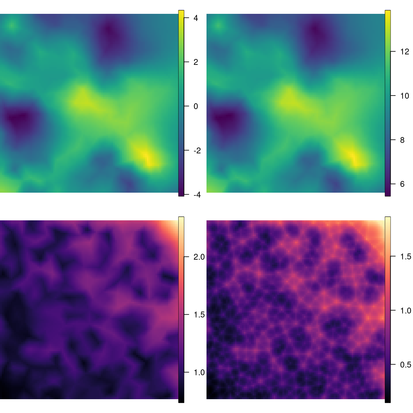
Figure 2.10: The mean and standard deviation of the random field (top left and bottom left, respectively) and the mean and standard deviation of the fitted values (top right and bottom right, respectively).
Figure 2.10 shows that there is a variation from -4 to 4 in the spatial effect. Considering also that standard deviations range from about 0.8 to 1.6, spatial dependence is considerable. In addition, the standard deviation of both the random field and \(\mu\) are smaller near corner (0, 0) and larger near corner (1, 1). This is just proportional to the locations density.
The two standard deviation fields are different because one is for the random field only and the other is for the expected value of the outcome, which takes into account the standard deviation of the mean as well.
2.5.4 Results from different meshes
In this section, results for the toy dataset based on the six different meshes
built in Section 2.6 will be compared. To do this comparison, the
posterior marginal distributions of the model parameters will be plotted. The
true values used in the simulation of the toy dataset have been added to the
plots in order to evaluate the impact of the meshes on the results. Also,
maximum likelihood estimates using the geoR package (Ribeiro Jr. and Diggle 2001) have been added.
Six models will be fitted, using each one of the six meshes, and the results are put together in a list using the following code:
lrf <- list()
lres <- list()
l.dat <- list()
l.spde <- list()
l.a <- list()

for (k in 1:6) {
  # Create A matrix
  l.a[[k]] <- inla.spde.make.A(get(paste0('mesh', k)),
    loc = coords)
  # Creeate SPDE spatial effect
  l.spde[[k]] <- inla.spde2.pcmatern(get(paste0('mesh', k)),
    alpha = 2, prior.range = c(0.1, 0.01),
    prior.sigma = c(10, 0.01))

  # Create list with data
  l.dat[[k]] <- list(y = SPDEtoy[,3], i = 1:ncol(l.a[[k]]),
    m = rep(1, ncol(l.a[[k]])))
  # Fit model
  lres[[k]] <- inla(y ~ 0 + m + f(i, model = l.spde[[k]]),
    data = l.dat[[k]], control.predictor = list(A = l.a[[k]]))
}
Mesh size influences the computational time needed to fit the model. More
nodes in the mesh need more computational time. The times required to fit the
models with INLA for these six meshes are shown in Table
2.1.
| Mesh | Size | Time |
|---|---|---|
| 1 | 2900 | 74.8375 |
| 2 | 488 | 1.3091 |
| 3 | 371 | 0.8305 |
| 4 | 2878 | 43.8911 |
| 5 | 490 | 1.5561 |
| 6 | 375 | 1.1386 |
Furthermore, the posterior marginal distribution of \(\sigma_e^2\) is computed for each fitted model:
s2.marg <- lapply(lres, function(m) {
  inla.tmarginal(function(x) exp(-x),
    m$internal.marginals.hyperpar[[1]])
})
The true values of the model parameters are: \(\beta_0=10\), \(\sigma_e^2=0.3\), \(\sigma_x^2=5\), range \(\sqrt{8}/7\) and \(\nu=1\). The \(\nu\) parameter is fixed at the true value as a result of setting \(\alpha=2\) in the definition of the SPDE model.
beta0 <- 10
sigma2e <- 0.3
sigma2u <- 5
range <- sqrt(8) / 7
nu <- 1
The maximum likelihood estimates obtained with package geoR (Ribeiro Jr. and Diggle 2001) are:
lk.est <- c(beta = 9.54, s2e = 0.374, s2u = 3.32,
  range = 0.336 * sqrt(8))
The posterior marginal distributions of \(\beta_0\), \(\sigma_e^2\), \(\sigma_x^2\), and range have been plotted in Figure 2.11. Here, it can be seen how the posterior marginal distribution of the intercept has its mode at the likelihood estimate, considering the results from all six meshes.
The main differences can be found in the noise variance \(\sigma_e^2\) (i.e., the nugget effect). The results from the mesh based on the points have a posterior mode which is smaller than the actual value and the maximum likelihood estimate. In general, as the number of triangles in the mesh increase, the posterior mode gets closer to the actual value of the parameter. Regarding the meshes computed from the boundary, they seem to provide posterior modes which are closer to the maximum likelihood estimate than the other meshes.
Regarding the marginal variance of the latent field, \(\sigma_x^2\), all meshes produced results in a posterior smaller than the actual value and closer to the maximum likelihood estimate. For the range, all meshes have a mode smaller than the maximum likelihood estimate and very close to the actual value.
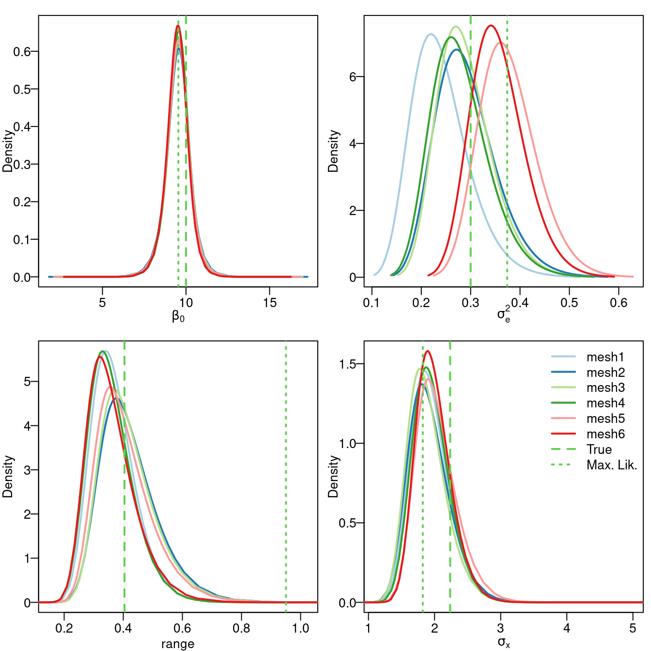
Figure 2.11: Marginal posterior distribution for \(\beta_0\) (top left), \(\sigma_e^2\) (top right), range (bottom left) and \(\sqrt{\sigma_x^2}\) (bottom right).
Although these results are based on a toy example and are not conclusive, a general comment is that it is good to have a mesh tuned about the point locations, to capture noise variance. It is also important to allow for some flexibility to avoid a large variability in the shape and size of the triangles, to get good estimates of the latent field parameters. Thus, it is a tradeoff between (1) point locations and (2) large variability in the shape of the mesh triangles.
2.6 Triangulation details and examples
As stated earlier in this chapter, the first step to fit an SPDE model is the construction of the mesh to represent the spatial process. This step must be done very carefully, since it is similar to choosing the integration points on a numeric integration algorithm. Should the points be taken at regular intervals? How many points are needed? Furthermore, additional points around the boundary, or outer extension, need to be chosen with care. This is necessary to avoid a boundary effect that may cause a variance twice as larger at the border than within the domain (Lindgren 2012; Lindgren and Rue 2015).
Finally, in order to experiment with mesh building, there is a Shiny
application in the INLA package that can be loaded with meshbuilder().
This will be useful to learn and understand how the different parameters
are used in the definition of the mesh work. This is further described in
Section 2.7.
2.6.1 Getting started
For a two dimensional mesh, function inla.mesh.2d() is the one that is
recommended to use for building a mesh. This function creates a Constrained
Refined Delaunay Triangulation (CRDT) over the study region, that will be simply
referred to as the mesh. This function can take several arguments:
str(args(inla.mesh.2d))
## function (loc = NULL, loc.domain = NULL, offset = NULL,
##     n = NULL, boundary = NULL, interior = NULL,
##     max.edge = NULL, min.angle = NULL, cutoff = 1e-12,
##     max.n.strict = NULL, max.n = NULL, plot.delay = NULL,
##     crs = NULL)
First of all, some information about the study region is needed to create the
mesh. This can be provided by the location points or just a domain. The point
locations, which can be passed to the function in the loc argument, are used
as initial triangulation nodes. A single polygon can be supplied to determine
the domain extent using the loc.domain argument. After the location
points or the boundary have been passed to the function, the algorithm will
find a convex hull mesh. A non-convex hull mesh can be made when a
list of polygons is passed using the boundary argument, where each element of
this list is of the class returned by function inla.mesh.segment(). Hence,
one of these three arguments (loc, domain or boundary) is mandatory.
The other mandatory argument is max.edge. This argument specifies the maximum
allowed triangle edge length in the inner domain and in the outer extension.
So, it can be a single numeric value or length two vector, and it must be in
the same scale units as the coordinates.
The other arguments are used to specify additional constraints on the mesh. The
offset argument is a numeric value (or a length two vector) and it is used to
set the automatic extension distance. If positive, it is the extension
distance in the same scale units. If
negative, it is interpreted as a factor relative to the approximate data
diameter; i.e., a value of -0.10 (the default) will add a 10% of the data
diameter as outer extension.
Argument n is the initial number of points in the extended boundary. The
interior argument is a list of segments to specify interior constraints, each
one of the inla.mesh.segment class. A good mesh needs to have triangles as
regular as possible in size and shape. This can be controlled with argument
max.edge to control the edge length of the triangles and the min.angle
argument (which can be scalar or length two vector) can be used to specify the
minimum internal angles of the triangles in the inner domain and the outer
extension. Values up to 21 guarantee the convergence of the algorithm
(de Berg et al. 2008; Guibas, Knuth, and Sharir 1992).
To further control the shape of the triangles, the cutoff argument can be
used to set the minimum allowed distance between points. It means that points
at a closer distance than the supplied value are replaced by a single vertex.
Hence, it avoids small triangles and must be a positive number, and is critical
when there are some points very close to each other, either for point locations
or in the domain boundary.
To understand how function inla.mesh.2d() works, several meshes have been
computed for different combinations of some of the arguments using the first
five locations of the toy dataset. First, the toy dataset will be loaded and
its first five points taken:
data(SPDEtoy)
coords <- as.matrix(SPDEtoy[, 1:2])
p5 <- coords[1:5, ]
As the meshes will be built using the domain and not the points, this domain needs to be defined first:
pl.dom <- cbind(c(0, 1, 1, 0.7, 0, 0), c(0, 0, 0.7, 1, 1, 0))This domain has been plotted in green over some of the meshes in Figure 2.12.
Finally, the meshes are created using the first five points or the domain defined above:
m1 <- inla.mesh.2d(p5, max.edge = c(0.5, 0.5))
m2 <- inla.mesh.2d(p5, max.edge = c(0.5, 0.5), cutoff = 0.1)
m3 <- inla.mesh.2d(p5, max.edge = c(0.1, 0.5), cutoff = 0.1)
m4 <- inla.mesh.2d(p5, max.edge = c(0.1, 0.5),
  offset = c(0, -0.65))
m5 <- inla.mesh.2d(loc.domain = pl.dom, max.edge = c(0.3, 0.5),
  offset = c(0.03, 0.5))
m6 <- inla.mesh.2d(loc.domain = pl.dom, max.edge = c(0.3, 0.5),
  offset = c(0.03, 0.5), cutoff = 0.1)
m7 <- inla.mesh.2d(loc.domain = pl.dom, max.edge = c(0.3, 0.5),
  n = 5, offset = c(0.05, 0.1))
m8 <- inla.mesh.2d(loc.domain = pl.dom, max.edge = c(0.3, 0.5),
  n = 7, offset = c(0.01, 0.3))
m9 <- inla.mesh.2d(loc.domain = pl.dom, max.edge = c(0.3, 0.5),
n = 4, offset = c(0.05, 0.3)) 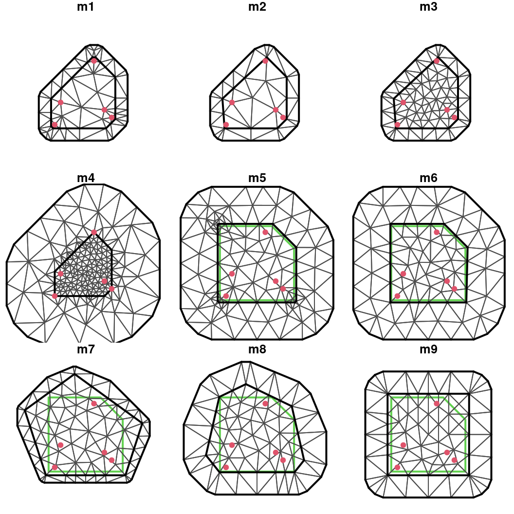
Figure 2.12: Different triangulations created with function inla.mesh.2d() using different combinations of its arguments.
These nine meshes have been displayed in Figure 2.12. In the next paragraphs we provide a comparative critical assessment of the quality of the different meshes depending on their structure.
The m1 mesh has two main problems. First, there are some triangles with
small inner angles and, second, some large triangles appear in the inner
domain. In the m2 mesh, the restriction on the locations is relaxed, because
points with distance less than the cutoff are considered a single vertex. This
avoids some of the triangles (at the bottom right corner) with small angles
that appeared in mesh m1. Hence, using a cutoff is a very good idea. Each
inner triangle in the m3 mesh has an edge length less than 0.1 and this mesh
looks better than the two previous ones.
The m4 mesh has been made without first building a convex hull extension
around the points. It has just the second outer boundary. In this case, the
length of the inner triangles is not good (first value in the max.edge
argument) and there are triangles with edge lengths of up to 0.5 in the outer
region. The shape of the triangles looks good in general.
The m5 mesh was made just using the domain polygon and it has a shape similar
to the domain area. In this mesh there are some small triangles at the corners
of the domain due to the fact that it has been built without specifying a
cutoff. Also, there is a (relatively) small first extension and a
(relatively) large second one. In the m6 mesh, a cutoff has been added and a
better mesh than the previous one has been obtained.
In the last three meshes, the initial number of extension points has been
changed. It can be useful to change this value in some situations to get a
convergence of the mesh building algorithm. For example, Figure
2.12 shows the shape of the mesh obtained with n = 5 in the m7 mesh. This number produces a mesh that seems inadequate for
this domain because there is a non uniform extension behind the border.
Meshes m8 and m9 have very bad triangle shapes.
The object returned by the inla.mesh.2d() function is of class inla.mesh
and it is a list with several elements:
class(m1)
## [1] "inla.mesh"
names(m1)
## [1] "meta"     "manifold" "n"        "loc"      "graph"
## [6] "segm"     "idx"      "crs"
The number of vertices in each mesh is in the n element of this list, which
allows us to compare the number of vertices of all the meshes created:
c(m1$n, m2$n, m3$n, m4$n, m5$n, m6$n, m7$n, m8$n, m9$n)
## [1]  61  36  79 195 117  88  87  69  72
The graph element represents the CRDT obtained. In addition, the graph
element contains the matrix that represents the graph of the neighborhood
structure. For example, for mesh m1 this matrix has the following dimension:
dim(m1$graph$vv)
## [1] 61 61
The vertices that correspond to the location points are identified in the idx
element:
m1$idx$loc
## [1] 24 25 26 27 28
2.6.2 Non-convex hull meshes
All meshes in Figure 2.12 have been made to have a convex hull
boundary. In this context, a convex hull is a polygon of triangles out of the
domain area, the extension made to avoid the boundary effect. A triangulation
without an additional border can be made by supplying the boundary argument
instead of the location or loc.domain arguments. One way to create a
non-convex hull is to build a boundary for the points and supply it in the
boundary argument.
Boundaries can also be created by using the inla.nonconvex.hull() function,
which takes the following arguments:
str(args(inla.nonconvex.hull))
## function (points, convex = -0.15, concave = convex,
##     resolution = 40, eps = NULL, crs = NULL)
When using this function, the points and a set of constraints need to be passed. The shape of the boundary can be controlled, including its convexity, concavity and resolution. In the next example, some boundaries are created first and then a mesh is built with each one to better understand how this process works:
# Boundaries
bound1 <- inla.nonconvex.hull(p5)
bound2 <- inla.nonconvex.hull(p5, convex = 0.5, concave = -0.15)
bound3 <- inla.nonconvex.hull(p5, concave = 0.5)
bound4 <- inla.nonconvex.hull(p5, concave = 0.5,
  resolution = c(20, 20))

# Meshes
m10 <- inla.mesh.2d(boundary = bound1, cutoff = 0.05,
  max.edge = c(0.1, 0.2))
m11 <- inla.mesh.2d(boundary = bound2, cutoff = 0.05,
  max.edge = c(0.1, 0.2))
m12 <- inla.mesh.2d(boundary = bound3, cutoff = 0.05,
  max.edge = c(0.1, 0.2))
m13 <- inla.mesh.2d(boundary = bound4, cutoff = 0.05,
  max.edge = c(0.1, 0.2))
These meshes have been displayed in Figure 2.13 and a discussion on the quality of the produced meshes is provided below.
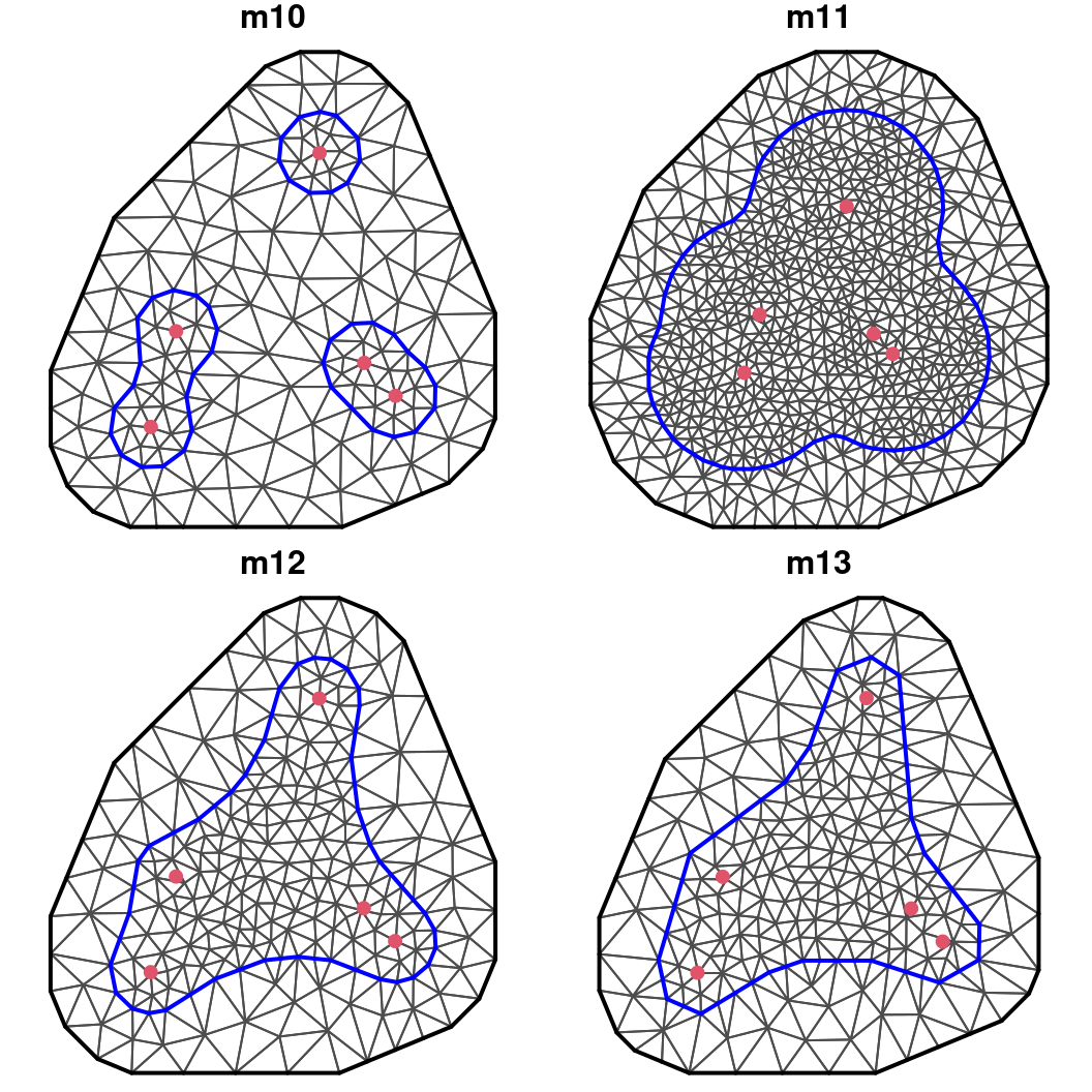
Figure 2.13: Non-convex meshes with different boundaries.
The m10 mesh is built with a boundary that uses the default arguments in the
inla.nonconvex.hull() function. The default convex and concave arguments
are both equal to a proportion of 0.15 of the points’ domain radius, that is
computed as follows:
0.15 * max(diff(range(p5[, 1])), diff(range(p5[, 2])))
## [1] 0.1291
If we supply a larger value in the convex argument, such as the one used to
generate mesh m11, a larger boundary is obtained. This happens because all
circles with a center at each point and a radius less than the convex value are
inside the boundary. When a larger value for the concave argument is taken,
as in the boundary used for the m12 and m13 meshes, there are no circles
with radius less than the concave value outside the boundary. If a smaller
resolution is chosen, a boundary with small resolution (in terms of number of
points) is obtained. For example, compare the m12 and m13 meshes.
2.6.3 Meshes for the toy example
To analyze the toy data set, six triangulation sets of options were used to make comparisons in Section 2.5.4. The first and second meshes force the location points to be vertices of the mesh, but the maximum length of the edges is allowed to be larger in the second mesh:
mesh1 <- inla.mesh.2d(coords, max.edge = c(0.035, 0.1))
mesh2 <- inla.mesh.2d(coords, max.edge = c(0.15, 0.2))
The third mesh is based on the points, but a cutoff greater than zero is taken to avoid small triangles in regions with a high number of observations:
mesh3 <- inla.mesh.2d(coords, max.edge = c(0.15, 0.2),
  cutoff = 0.02)
Three other meshes have been created based on the domain area. These are built to have approximately the same number of vertices as the previous ones:
mesh4 <- inla.mesh.2d(loc.domain = pl.dom,
  max.edge = c(0.0355, 0.1))
mesh5 <- inla.mesh.2d(loc.domain = pl.dom,
  max.edge = c(0.092, 0.2))
mesh6 <- inla.mesh.2d(loc.domain = pl.dom,
  max.edge = c(0.11, 0.2))
These six meshes are shown in Figure 2.14. The number of nodes in each one of these meshes is:
c(mesh1$n, mesh2$n, mesh3$n, mesh4$n, mesh5$n, mesh6$n)
## [1] 2900  488  371 2878  490  375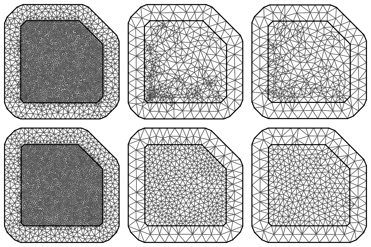
Figure 2.14: Six triangulations with different options for the toy example.
2.6.4 Meshes for Paraná state
In this book there are some examples using data collected in Paraná state, Brazil. In order to build a mesh to represent this region, two things need to be taken into account: the shape of this domain area and its coordinate reference system.
First of all, the daily rainfall dataset will be loaded (as this contains the boundary of Paraná state that can be used in the analysis):
data(PRprec)This dataset comprises daily rainfall data from 616 stations in the 2011 year. The coordinates (two first columns) are in longitude and latitude. Altitude of the station is under the third column. Hence, the dimension of the data is:
dim(PRprec)
## [1] 616 368
The coordinates and data for the first 5 days of the year of the first two stations can be seen below to get an idea of the information available in this dataset:
PRprec[1:2, 1:8]
##   Longitude Latitude Altitude d0101 d0102 d0103 d0104 d0105
## 1    -50.87   -22.85      365     0     0     0     0     0
## 3    -50.77   -22.96      344     0     1     0     0     0
Also, boundaries of Paraná state as a polygon are available:
data(PRborder)
dim(PRborder)
## [1] 2055    2
This is a set of 2055 points, in longitude and latitude.
As the boundary is irregular, in this case it is best to use a non-convex hull mesh. The first step is to build a non-convex domain using the locations of the precipitation data, as follows:
prdomain <- inla.nonconvex.hull(as.matrix(PRprec[, 1:2]),
  convex = -0.03, concave = -0.05,
  resolution = c(100, 100))
Using this defined domain, two meshes will be built with different resolutions (i.e., different maximum edge lengths) in the inner domain:
prmesh1 <- inla.mesh.2d(boundary = prdomain,
  max.edge = c(0.7, 0.7), cutoff = 0.35,
   offset = c(-0.05, -0.05))
prmesh2 <- inla.mesh.2d(boundary = prdomain,
  max.edge = c(0.45, 1), cutoff = 0.2)
The number of points in each mesh is 187 and 382, respectively. Both meshes have been displayed in Figure 2.15.
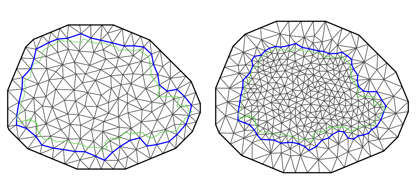
Figure 2.15: Meshes for Paraná state (Brazil).
2.6.5 Triangulation with a SpatialPolygonsDataFrame
Sometimes, the domain region is available as a map in some GIS format. In
R, a widely used representation of a spatial object is made using object
classes in the sp package (Bivand, Pebesma, and Gomez-Rubio 2013). To show an application in this
case, the North Carolina map, which is extensively analyzed in the examples in
package spdep (Bivand and Piras 2015), will be used. Shapefiles of North Carolina
are currently available in package spData (Bivand, Nowosad, and Lovelace 2018).
First of all, the map will be loaded using function readOGR() from package
rgdal (R. Bivand, Keitt, and Rowlingson 2017):
library(rgdal)
# Get filename of file to load
nc.fl <- system.file("shapes/sids.shp", package = "spData")[1]
# Load shapefile
nc.sids <- readOGR(strsplit(nc.fl, 'sids')[[1]][1], 'sids')
This map contains the boundaries of the different counties in North Carolina.
For this reason, this map is simplified by uniting all the county areas
together in order to get the outer boundary of North Carolina. To do it, the
gUnaryUnion() function from the rgeos package (R. Bivand and Rundel 2017) is used:
library(rgeos)
nc.border <- gUnaryUnion(nc.sids, rep(1, nrow(nc.sids)))
Now, the inla.sp2segment() function is used to extract the boundary of the
SpatialPolygons object that contains the boundary of the map:
nc.bdry <- inla.sp2segment(nc.border)Then, the mesh is finally created and it has been displayed in Figure 2.16:
nc.mesh <- inla.mesh.2d(boundary = nc.bdry, cutoff = 0.15,
  max.edge = c(0.3, 1))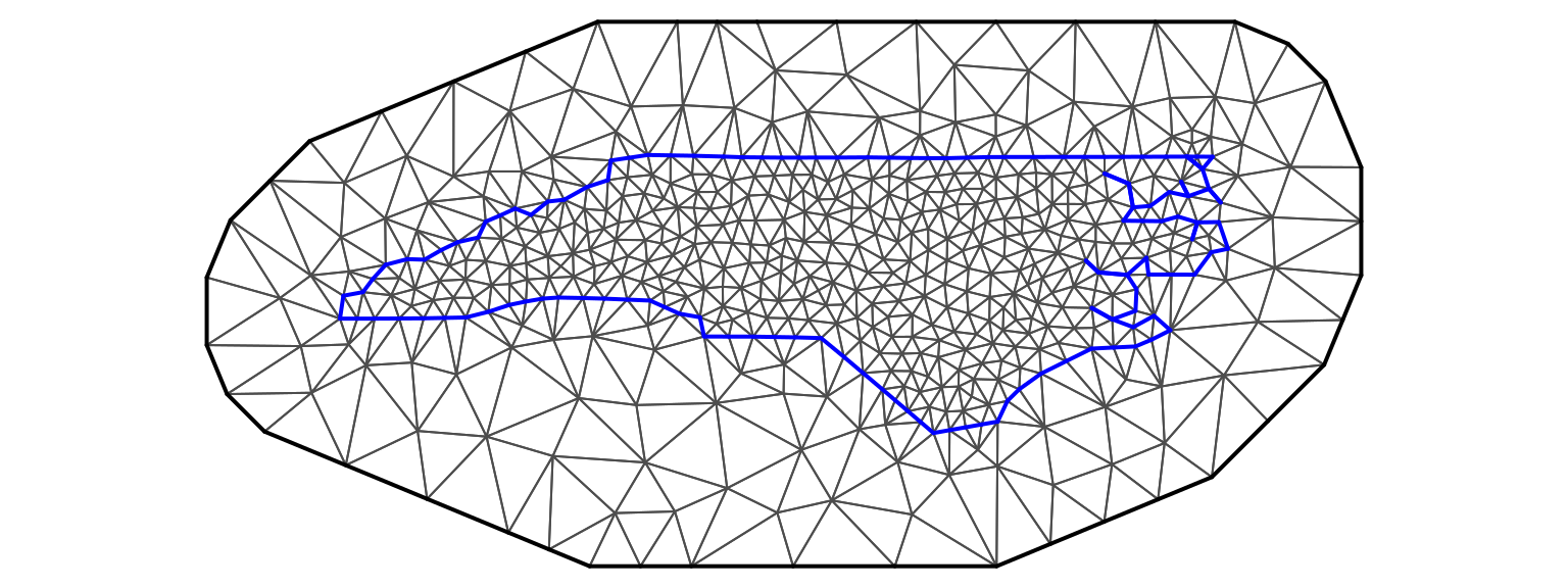
Figure 2.16: Mesh constructed using the North Carolina map.
2.6.6 Mesh with holes and physical boundaries
So far, the domains considered in the analysis were simply connected because they did not contain any holes. However, sometimes we may find that the spatial process under study occurs in a domain which contain holes. These holes also produce physical boundaries that need to be taken into account in the analysis.
An example of application is when modeling fish and inland is required to be considered as a physical barrier. In addition, islands in the study region will be required to be taken into account. Similarly, when studying species distribution in a forest, lakes and rivers may introduce natural barriers that also need to be taken into account. These types of models are further described in Chapter 5.
The polygons in Figure 2.17 illustrate this case, as they include a hole in the left polygon. These polygons have been created with the following commands:
pl1 <- Polygon(cbind(c(0, 15, 15, 0, 0), c(5, 0, 20, 20, 5)),
  hole = FALSE)
h1 <- Polygon(cbind(c(5, 7, 7, 5, 5), c(7, 7, 15, 15, 7)),
  hole = TRUE)
pl2 <- Polygon(cbind(c(15, 20, 20, 30, 30, 15, 15),
  c(10, 10, 0, 0, 20, 20, 10)), hole = FALSE)
sp <- SpatialPolygons(
  list(Polygons(list(pl1, h1), '0'), Polygons(list(pl2), '1')))
Here, pl1 corresponds to the left polygons, with a hole defined by polygon
h1, and pl2 is the polygon on the right. All these three polygons are
combined into a SpatialPolygons object called sp.
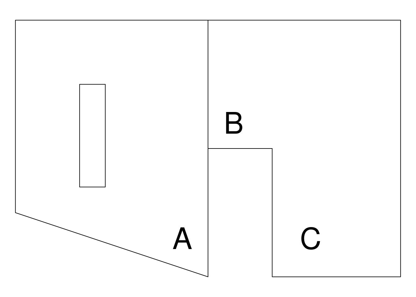
Figure 2.17: Region with a hole and non-convex domain.
Hence, there are two neighboring regions, one with a hole and another one with no convex shape. Let us consider that the two polygons represent two regions in a lake with their outer boundaries representing the shore and with the hole on the left representing an island. Suppose that it is necessary to avoid correlation between near regions separated by land. For example, suppose that correlation between A and C should be smaller than between A and B or between B and C.
In this example, additional points for the outer boundary are not needed. For
this reason, a length one value for max.edge must be passed. The following
code prepares the boundary and builds the mesh:
bound <- inla.sp2segment(sp)
mesh <- inla.mesh.2d(boundary = bound, max.edge = 2)
The mesh is displayed in Figure 2.18. Notice that when building the SPDE model, the neighborhood structure of the mesh is taken into account. In this case, it is easier to reach B from A than to reach B from C on the related graph. Hence, the SPDE model will consider a higher correlation between B and A than between B and C.
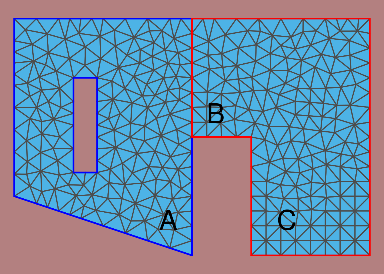
Figure 2.18: Triangulation with hole and a non-convex region.
2.7 Tools for mesh assessment
Building the right mesh for a spatial model may require some tuning and time.
For this reason, INLA includes a Shiny (Chang et al. 2018) application that can be
used to set the parameters interactively and display the resulting mesh in a
few seconds. Figure 2.19 shows the Shiny application, which
can be run with:
meshbuilder()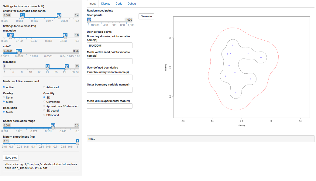
Figure 2.19: Shiny application to interactively create a mesh obtained with command meshbuilder().
The mesh builder has a number of options to define the mesh on the left side.
These include options to be passed to functions inla.nonconvex.hull() and
inla.mesh.2d() and the resulting mesh displayed on the right part. Below
these options, there are a number of options to assess the mesh resolution.
These include a number of quantities to be plotted, such as the standard
deviation (SD).
The right part of the application has four tabs that can be clicked to show
different outputs. By default, the application opens the Input tab,
which includes options to set the points and, possibly, boundaries to create
the mesh.
The Display tab shows the created mesh, as well as some information about it
at the bottom. If option Active under Mesh resolution assessment has been
clicked, then this plot will also show the variable marked under Quantity. By
selecting different quantities, it is possible to assess how the created mesh
will produce the estimates from the model. Figure 2.20 shows
the generated mesh as well as the point values of the model standard deviation.
Note how the higher values appear in the outer region, which is close to the mesh
boundary and outside the domain of interest.
By including this outer region the estimates of the spatial
process in the study region do not suffer from any boundary effect.
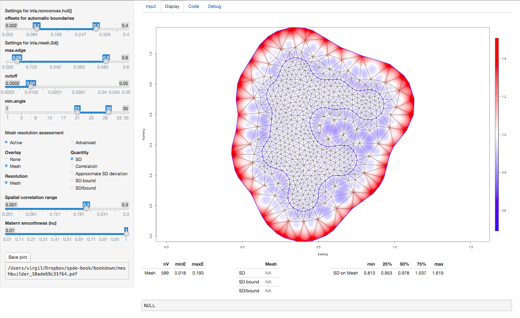
Figure 2.20: Display of the estimated standard deviation of the spatial process under the Display tab in the Shiny application.
The next tab, is the Code tab. This will show the R code used to generate
the mesh. Finally, the Debug tab provides some internal debugging information.
2.8 Non-Gaussian response: Precipitation in Paraná
Now, more complex spatial models based on the SPDE approach will be considered. In particular, the analysis of non-Gaussian observations, which will be illustrated using rainfall data from Paraná (Brazil).
Climate data is a very common type of spatial data. The example data we will use here is collected by the National Water Agency in Brazil (Agencia Nacional de Águas, ANA, in Portuguese). ANA collects data from many locations over Brazil, and all these data are freely available from the ANA website (http://www3.ana.gov.br/portal/ANA).
2.8.1 The data set
As mentioned in Section 2.6.4, this dataset is composed
of daily rainfall data from year 2011 at 616 locations, including stations
within Paraná state and around its border. This dataset is available in the
INLA package and it can be loaded as follows:
data(PRprec) The coordinates of the locations where the data were collected are in the first two columns, altitude is next in the third column and the following 365 columns, one for each day of the year, store the daily accumulated precipitation.
In the code below the first eight columns from four stations of the PRprec
dataset are shown. These four stations (defined in index ii) are the one with
the lowest latitude (among all stations with missing altitude), the ones with
the lowest and largest longitude and the one with the highest altitude.
ii <- c(537, 304, 610, 388)
PRprec[ii, 1:8]
##      Longitude Latitude Altitude d0101 d0102 d0103 d0104 d0105
## 1239    -48.94   -26.18       NA  20.5   7.9   8.0   0.8   0.1
## 658     -48.22   -25.08        9  18.1   8.1   2.3  11.3  23.6
## 1325    -54.48   -25.60      231  43.8   0.2   4.6   0.4   0.0
## 885     -51.52   -25.73     1446   0.0  14.7   0.0   0.0  28.1
These four stations have been represented using red crosses in the right plot in Figure 2.21.
There are a few problems with this dataset. First of all, there are seven stations with missing altitude and missing data on daily rainfall, which are displayed in red in the left plot in Figure 2.21. If altitude is considered when building a model it will be important to have this variable measured everywhere in the state. There are digital elevation models that can be considered to find out the altitude at these locations. Alternatively, a stochastic model for this variable can be considered.
Daily rainfall mean in January 2011 will be considered in the analysis. However, there are 269 missing observations. As a simple imputation method, the average over the number of days in January 2011 without missing data will be taken, as follows:
PRprec$precMean <- rowMeans(PRprec[, 3 + 1:31], na.rm = TRUE)
summary(PRprec$precMean)
##    Min. 1st Qu.  Median    Mean 3rd Qu.    Max.    NA's
##    0.50    4.97    6.54    6.96    8.63   21.66       6
There are still some stations with missing values of the monthly average in January 2011. The number of missing observations in July 2011 at each station can be checked as:
table(rowSums(is.na(PRprec[, 3 + 1:31])))
##
##   0   2   4   8  17  26  31
## 604   1   1   1   1   2   6
Hence, there are some stations with all the observations missing during January 2011, and this is the reason why the average during January 2011 is also missing.
In addition to the rainfall data, the Paraná state border will also be considered to define the study domain:
data(PRborder) The locations of the data are displayed in Figure 2.21. The size of the points on the left plot is proportional to the altitude at the locations. The cyan line in the east border is the coast (along the Atlantic Ocean). There are low altitudes near the ocean, and high altitudes around 50 to 100 kilometers from this coast and from the center of the state towards the south as well. Altitude decreases to the north and west sides of Paraná state. The size of the points in the right plot is proportional to the daily average of the precipitation in January 2011. In this case, there are higher values near the coast.
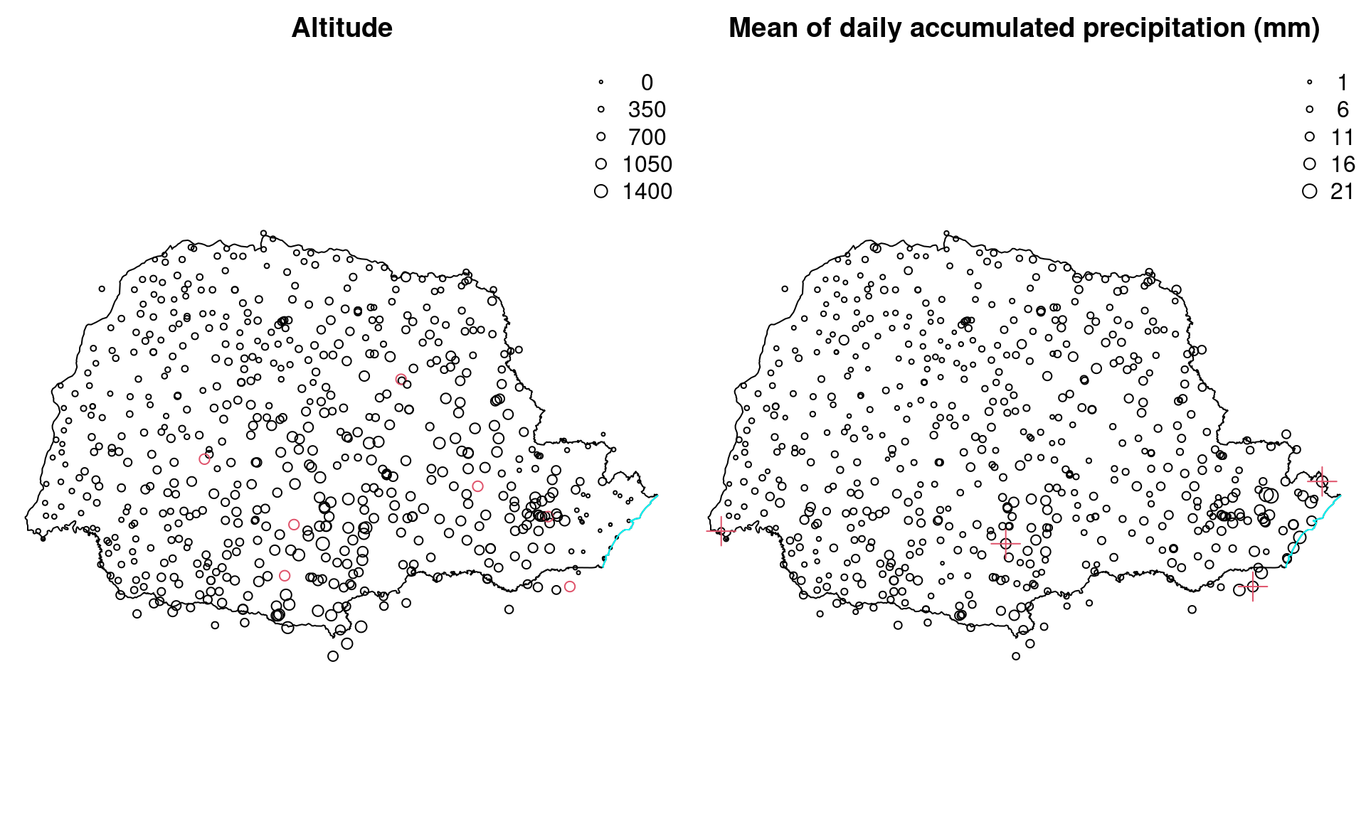
Figure 2.21: Locations of Paraná stations, altitude and average of daily accumulated precipitation (mm) in January 2011. Circles in red denote stations with missing observations and red crossess denote the four stations shown in the example in the main text.
2.8.2 Model and covariate selection
In this section the average of the daily accumulated precipitation for each of the 31 days in January 2011 will be analyzed. Given that it must be a positive value, a Gamma likelihood will be considered. In the Gamma likelihood, the mean is \(E(y_i) = a_i/b_i = \mu_i\) and the variance is \(V(y_i) = a_i/b_i^2 = \mu_i^2/\phi\), where \(\phi\) is a precision parameter. Then it is necessary to define a model for the linear predictor \(\eta_i = \log(\mu_i)\), which will depend on the covariates \(\mathbf{F}\) and the spatial random field \(\mathbf{x}\) as follows:
\[ \begin{array}{rcl} y_i|\mathbf{F_i},\alpha,x_i,\theta & \sim & Gamma(a_i, b_i) \\ log(\mu_i) & = & \alpha + f(\mathbf{F_i}) + x_i\\ \mathbf{x} & \sim & GF(0, \Sigma) \end{array} \]
Here, \(\mathbf{F_i}\) is a vector of covariates (the location coordinates and altitude of station \(i\)) that will be assumed to follow a function detailed later and \(\mathbf{x}\) is the spatial latent Gaussian random field (GF). For this, a Matérn covariance function will be considered with parameters \(\nu\), \(\kappa\) and \(\sigma_x^2\).
2.8.2.1 Smoothed covariate effect
An initial exploration of the relationship between precipitation and the other covariates has been made by means of dispersion diagrams, available in Figure 2.22. After preliminary tests, it seems reasonable to construct a new covariate: the distance from each station to the Atlantic Ocean. The Paraná state border along the Atlantic Ocean is shown as a cyan line in Figure 2.21. The minimum distance from each station to this line can be computed to obtain the distance from the station to the Atlantic Ocean.
To have this distance in kilometers the spDists() function from the sp
package will be used (with argument longlat equal to TRUE):
coords <- as.matrix(PRprec[, 1:2])
mat.dists <- spDists(coords, PRborder[1034:1078, ],
  longlat = TRUE)
However, this function computes the distance between each location in the first set of points to each point in the second set of points. So, the minimum value along the rows of the resulting matrix of distances must be taken to obtain the minimum distance to the ocean:
PRprec$oceanDist <- apply(mat.dists, 1, min) The dispersion plots can be seen in Figure 2.22. The average precipitation seems to have a well defined non-linear relationship with longitude. Also, there is a similar, but inverse, relation with distance to the ocean. Hence, two models will be built. The first one will include longitude as a covariate and the second one will include distance to the ocean. Model fitting measures will be computed to proceed with model choice between these two options.
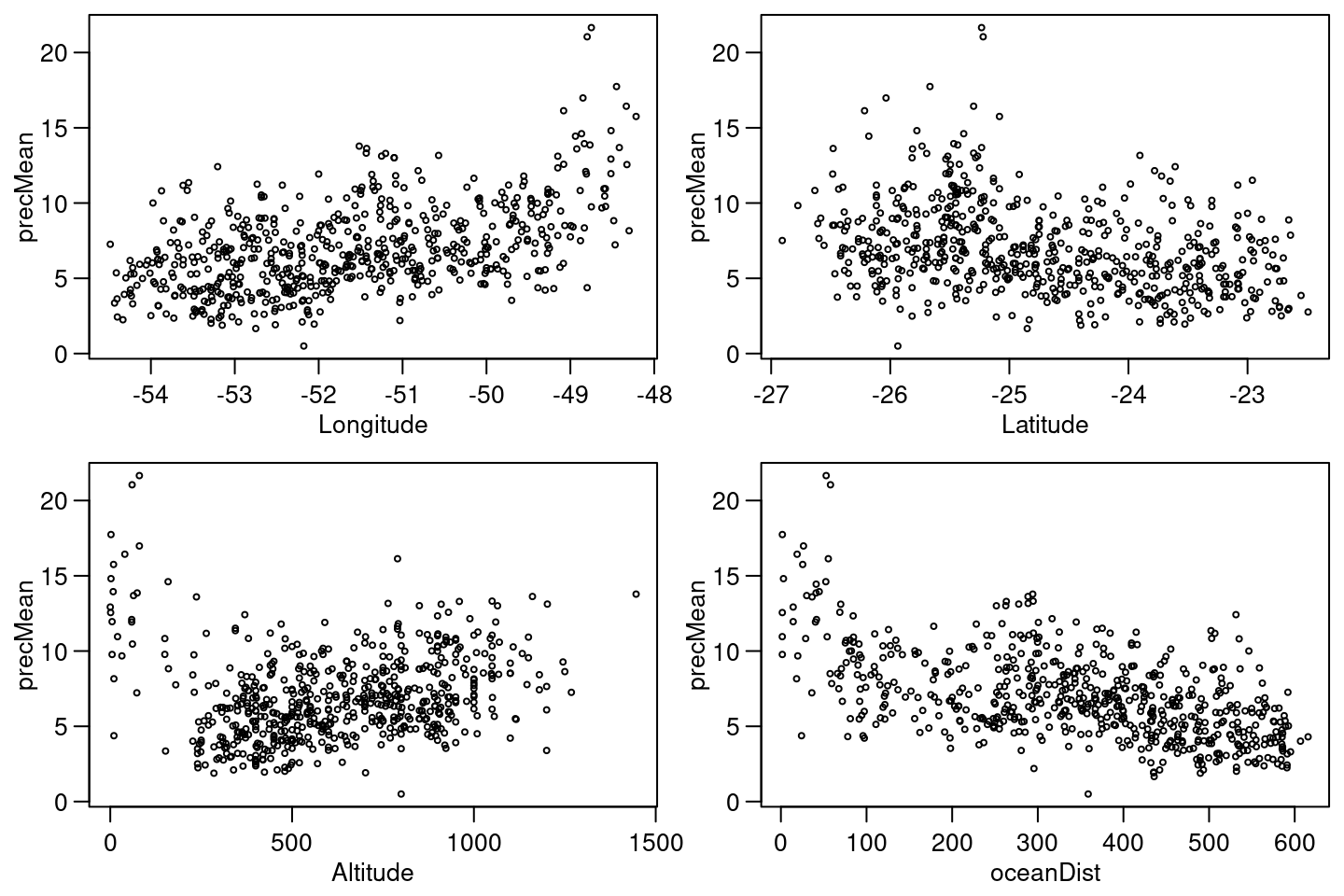
Figure 2.22: Dispersion plots of average of daily accumulated precipitation by longitude (top left), latitude (top right), altitude (bottom left) and distance to ocean (bottom right).
To consider a non-linear relationship for a covariate a random walk prior on
its effect can be set. To do that, the covariate can be discretized into a set
of knots and the random walk prior placed on them. In this case, the term in
the linear predictor due to ocean distance (or longitude) is discretized into
\(m\) classes considering the inla.group() function. The model can be chosen
from any one dimensional model available in INLA, such as rw1, rw2, ar1
or others. It can also be modeled using a one-dimensional Matérn model.
When considering intrinsic models as prior distributions, scaling the model
should be considered (Sørbye and Rue 2014). After scaling, the precision parameter
can be interpreted as the inverse of the random effect marginal variance.
Hence, scaling makes the process of defining a prior easier. The suggestion
here is to consider the PC-prior (Simpson et al. 2017) introduced in
Section 1.6.5. This can be done
by defining a reference standard deviation \(\sigma_0\) and the right tail
probability \(u\) as \(P(\sigma > \sigma_0) = u\). In this example,
these values will be set to \(\sigma_0 = 1\) and \(u = 0.01\). These
values can be stored in a list (to be passed to inla() later) as follows:
pcprec <- list(prior = 'pcprec', param = c(1, 0.01))2.8.2.2 Define the spatial model and prepare the data
In order to define the spatial model a mesh must be defined. First, a boundary around the points will be defined using a non-convex hull and used to create the mesh:
pts.bound <- inla.nonconvex.hull(coords, 0.3, 0.3)
mesh <- inla.mesh.2d(coords, boundary = pts.bound,
  max.edge = c(0.3, 1), offset = c(1e-5, 1.5), cutoff = 0.1)
Once the mesh has been defined, the projector matrix is computed:
A <- inla.spde.make.A(mesh, loc = coords)The SPDE model considering the PC-prior derived in Fuglstad et al. (2018) for the model parameters as the practical range, \(\sqrt{8\nu}/\kappa\), and the marginal standard deviation is defined as follows:
spde <- inla.spde2.pcmatern(mesh = mesh,
  prior.range = c(0.05, 0.01), # P(practic.range < 0.05) = 0.01
  prior.sigma = c(1, 0.01)) # P(sigma > 1) = 0.01
The stack data is defined to include four effects:
the GF, the intercept, longitude and distance to the ocean. The
R code to do this is:
stk.dat <- inla.stack(
  data = list(y = PRprec$precMean),
  A = list(A,1),
  effects = list(list(s = 1:spde$n.spde),
    data.frame(Intercept = 1,
      gWest = inla.group(coords[, 1]),
      gOceanDist = inla.group(PRprec$oceanDist),
      oceanDist = PRprec$oceanDist)),
  tag = 'dat')
2.8.2.3 Fitting the models
Both models will be fitted using the same data stack as only the formula needs
to be changed. For the model with longitude, the R code for model fitting
is:
f.west <- y ~ 0 + Intercept + # f is short for formula
  f(gWest, model = 'rw1', # first random walk prior
    scale.model = TRUE, # scaling this random effect
    hyper = list(prec = pcprec)) + # use the PC prior
  f(s, model = spde)

r.west <- inla(f.west, family = 'Gamma', # r is short for result
  control.compute = list(cpo = TRUE),
  data = inla.stack.data(stk.dat),
  control.predictor = list(A = inla.stack.A(stk.dat), link = 1))
Option link = 1 in the control.predictor is used to set the function link
to be considered in the computation of the fitted values that form the vector of available links for the Gamma likelihood:
inla.models()$likelihood$gamma$link
## [1] "default"  "log"      "quantile"
We recommend always using link = 1 if you do not have several likelihoods.
This will use the default link (i.e., the natural logarithm), but other link
functions can be used by changing the value of link.
For the model with distance to the ocean, the necessary code is:
f.oceanD <- y ~ 0 + Intercept +
  f(gOceanDist, model = 'rw1', scale.model = TRUE,
    hyper = list(prec = pcprec)) +
  f(s, model = spde)

r.oceanD <- inla(f.oceanD, family = 'Gamma',
  control.compute = list(cpo = TRUE),
  data = inla.stack.data(stk.dat),
  control.predictor = list(A = inla.stack.A(stk.dat), link = 1))
In Figure 2.23 it can be seen how the effect from distance to the ocean is almost linear. Hence, another model considering this linear effect has been fitted:
f.oceanD.l <- y ~ 0 + Intercept + oceanDist +
  f(s, model = spde)
r.oceanD.l <- inla(f.oceanD.l, family = 'Gamma',
  control.compute = list(cpo = TRUE),
  data = inla.stack.data(stk.dat),
  control.predictor = list(A = inla.stack.A(stk.dat), link = 1))
2.8.2.4 Model comparison and results
The negative sum of the log CPO (Pettit 1990, see Section 1.4) can be computed for each model using the following function:
slcpo <- function(m, na.rm = TRUE) {
  - sum(log(m$cpo$cpo), na.rm = na.rm)
}
Then, it can be used to compute this criterion for the three fitted models:
c(long = slcpo(r.west), oceanD = slcpo(r.oceanD),
  oceanD.l = slcpo(r.oceanD.l))
##     long   oceanD oceanD.l
##     1279     1279     1274
These results suggest that the model with distance to the ocean as a linear effect has a better fit than the other two models. This is just one way to show how to compare models considering how they fit the data. In this case, the three models have a very similar sum of the log CPO.
For the model with the best fit, a summary of the posterior distribution of the intercept and the covariate coefficient can be obtained with:
round(r.oceanD.l$summary.fixed, 2)
##           mean   sd 0.025quant 0.5quant 0.975quant mode kld
## Intercept 2.43 0.09       2.25     2.43       2.62 2.42   0
## oceanDist 0.00 0.00       0.00     0.00       0.00 0.00   0
Similarly, summaries for the Gamma likelihood dispersion parameter can be obtained:
round(r.oceanD.l$summary.hyperpar[1, ], 3)
##                                                 mean    sd
## Precision parameter for the Gamma observations 14.92 1.497
##                                                0.025quant
## Precision parameter for the Gamma observations      12.15
##                                                0.5quant
## Precision parameter for the Gamma observations    14.87
##                                                0.975quant
## Precision parameter for the Gamma observations      18.03
##                                                 mode
## Precision parameter for the Gamma observations 14.79
The summaries for the standard deviation and the practical range of the spatial process are:
round(r.oceanD.l$summary.hyperpar[-1, ], 3)
##              mean    sd 0.025quant 0.5quant 0.975quant  mode
## Range for s 0.662 0.142      0.436    0.644      0.988 0.607
## Stdev for s 0.234 0.022      0.193    0.233      0.280 0.231
Figure 2.23 displays the posterior marginals and estimates of some of the parameters in the previous models. For the model that considers a linear effect on the distance to the ocean, Figure 2.23 includes the posterior marginal distribution of the intercept \(\beta_0\), the coefficient of the distance to the ocean, the precision of the Gamma likelihood, and the range (in degrees) and standard deviation of the spatial effect. In order to compare the smooth term on the distance to the ocean, the top-left plot in Figure 2.23 shows the estimate of this effect using a random walk of order 1. As can be seen, this effect looks like a linear effect, and this is the reason why the model that considers a linear effect on distance to the ocean provides a better fit.
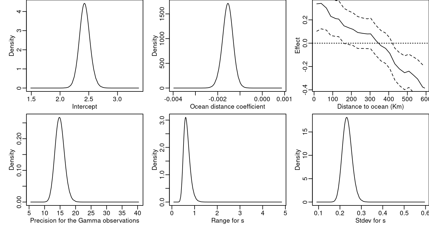
Figure 2.23: Posterior marginal distributions for \(\beta_0\) (top left), the distance to ocean coefficient (top center), the Gamma likelihood precision (bottom left), the practical range (bottom center) and the standard deviation of the spatial field (bottom right). The top-right plot represents the posterior mean (continuous line) and 95% credibility interval (dashed lines) for the distance to ocean effect.
If the significance of the spatial random effect component in the model needs to be assessed, a model without this term can be fitted. Then, the sum of the log CPO of these two models can be compared. A model without the spatial term can be fitted as follows:
r0.oceanD.l <- inla(y ~ 0 + Intercept + oceanDist,
  family = 'Gamma', control.compute = list(cpo = TRUE),
  data = inla.stack.data(stk.dat),
  control.predictor = list(A = inla.stack.A(stk.dat), link = 1))
In order to compare the negative sum of the log CPO, the following
R can be useful:
c(oceanD.l = slcpo(r.oceanD.l), oceanD.l0 =  slcpo(r0.oceanD.l))
##  oceanD.l oceanD.l0
##      1274      1371
Given these results, it can be concluded that the best model is the one that includes the spatial term and a linear effect on the distance to the ocean.
2.8.3 Prediction of the random field
The spatial effect can be visualized by projecting it on a grid. A regular grid will be considered so that each pixel is a square with a side of about 4 kilometers. A step of 4/111 will be used because each degree has approximately 111 kilometers, so that the size of the pixels can be given in degrees. Then, the step size is defined as:
stepsize <- 4 * 1 / 111As seen in Figure 2.21, the shape of Paraná state is wider along the x-axis than the y-axis and this fact will be considered when defining the grid. First, the range along each axis will be computed and then the size of the pixels will be used to set the number of pixels in each direction. We will divide the range along each axis by the step size and round it (to obtain integer values of the number of pixels in each direction):
x.range <- diff(range(PRborder[, 1]))
y.range <- diff(range(PRborder[, 2]))
nxy <- round(c(x.range, y.range) / stepsize)
Hence, the number of pixels in each direction is:
nxy
## [1] 183 117
The inla.mesh.projector() function will create a projector matrix. If a set
of coordinates is not supplied it will create a grid automatically. In the
next example, the limits and dimension of the grid are set as desired to match
the boundaries of Paraná state:
projgrid <- inla.mesh.projector(mesh, xlim = range(PRborder[, 1]),
  ylim = range(PRborder[, 2]), dims = nxy)
Then, this can be passed on to the inla.mesh.project() function to do the
projection of the posterior mean and the posterior standard deviation:
xmean <- inla.mesh.project(projgrid,
  r.oceanD$summary.random$s$mean)
xsd <- inla.mesh.project(projgrid, r.oceanD$summary.random$s$sd)
To improve the visualization, the pixels that fall outside Paraná state will be
assigned a value of NA. Points outside the state boundaries can be found
with function inout() from the splancs package (Rowlingson and Diggle 1993, 2017), as
follows:
library(splancs)
xy.in <- inout(projgrid$lattice$loc, PRborder)
Points with a value of TRUE will be those inside the boundaries of Paraná
state. The number of points in the grid inside and outside can be computed
with:
table(xy.in)
## xy.in
## FALSE  TRUE
##  7865 13546
Finally, the points that fall outside the boundaries are set to have a missing value of the posterior mean and standard deviation:
xmean[!xy.in] <- NA
xsd[!xy.in] <- NA
The posterior mean and posterior standard deviation for the spatial effect at each pixel can be seen in Figure 2.24. In the top left plot it can be seen that the posterior mean varies from \(-0.6\) to \(0.5\). This is the variation after accounting for the effect of the distance to the ocean. When comparing it to the standard deviation plot, these values seem to be considerable as the standard deviations takes a maximum value of about \(0.2\). The variation in the standard deviation is mainly due to the density of the stations over the region. At the top right plot in Figure 2.24, the first zone of high values from right to left is near the capital city of Curitiba, where the number of stations around is relatively larger than in any other regions of the state.
2.8.4 Prediction of the response on a grid
When the objective is to predict the response, a simple approach will be to add all the other terms to the spatial field projected in the previous section and apply the inverse of the link function. A full Bayesian analysis for this problem will involve computing the joint prediction of the response together with the estimation of the model, as in the first example below. However, it can be computationally expensive when the number of pixels in the grid is large. For this reason, we consider different options here, including a cheap way for the specific case in the second example below.
2.8.4.1 By computation of the posterior distributions
Considering the grid over Paraná state from the previous section, it can be avoided to compute the posterior marginal distributions at those pixels that are not inside the state boundaries. That is, only the lines in the projector matrix corresponding to points inside the state will be considered:
Aprd <- projgrid$proj$A[which(xy.in), ]The covariates for each pixel in the grid are needed now. In order to have them, the coordinates can be extracted from the projector object as well:
prdcoo <- projgrid$lattice$loc[which(xy.in), ]Computing the distance to the ocean for each selected pixel is easy:
oceanDist0 <- apply(spDists(PRborder[1034:1078, ],
  prdcoo, longlat = TRUE), 2, min)
Suppose that the model to be fitted is the one with the smoothed effect of distance to the ocean. Each computed distance needs to be discretized in the same way as for the estimation data at the stations. First of all, the used knots need to be obtained and ordered:
OcDist.k <- sort(unique(stk.dat$effects$data$gOceanDist))The knots are actually the middle values of the breaks and they will be considered as follows:
oceanDist.b <- (OcDist.k[-1] + OcDist.k[length(OcDist.k)]) / 2Next, each distance to the ocean computed for a pixel needs to be matched to a knot and this knot assigned to the pixel:
i0 <- findInterval(oceanDist0, oceanDist.b) + 1
gOceanDist0 <- OcDist.k[i0]
Building the data stack with the prediction data and joining it to the data with the data for estimation can be done as follows:
stk.prd <- inla.stack(
  data = list(y = NA),
  A = list(Aprd, 1),
  effects = list(s = 1:spde$n.spde,
    data.frame(Intercept = 1, oceanDist = oceanDist0)),
  tag = 'prd')
stk.all <- inla.stack(stk.dat, stk.prd)
When fitting the model for prediction, the mode of the hyperparameters (i.e.,
theta) obtained in the previous model can be passed as known values to the
new inla() call. It is also possible to avoid computing quantities not
needed, such as quantiles, and avoid returning objects not needed, such as the
posterior marginal distributions for the random effects and the linear
predictor. Since the number of latent variables is the main issue in this
case, the adaptive approximation will reduce computation time. It can be
set using control.inla = list(strategy = 'adaptive'). Only random
effects will get an adaptive approximation; any fixed effects are still
approximated with the simplified Laplace method.
Hence, the code to fit the model with the previous settings is:
r2.oceanD.l <- inla(f.oceanD.l, family = 'Gamma',
  data = inla.stack.data(stk.all),
  control.predictor = list(A = inla.stack.A(stk.all),
    compute = TRUE, link = 1),
  quantiles = NULL,
  control.inla = list(strategy = 'adaptive'),
  control.results = list(return.marginals.random = FALSE,
    return.marginals.predictor = FALSE),
  control.mode = list(theta = r.oceanD.l$mode$theta,
    restart = FALSE))
As in other examples, it is necessary to find the indices for the
predictions in the grid. It can be done by using the inla.stack.index()
function. These values must be assigned into the right positions of a matrix
with the same dimension as the grid. This is required for both the posterior
predicted mean and its standard deviation:
id.prd <- inla.stack.index(stk.all, 'prd')$data
sd.prd <- m.prd <- matrix(NA, nxy[1], nxy[2])
m.prd[xy.in] <- r2.oceanD.l$summary.fitted.values$mean[id.prd]
sd.prd[xy.in] <- r2.oceanD.l$summary.fitted.values$sd[id.prd]
The results are displayed in the bottom row of Figure 2.24.
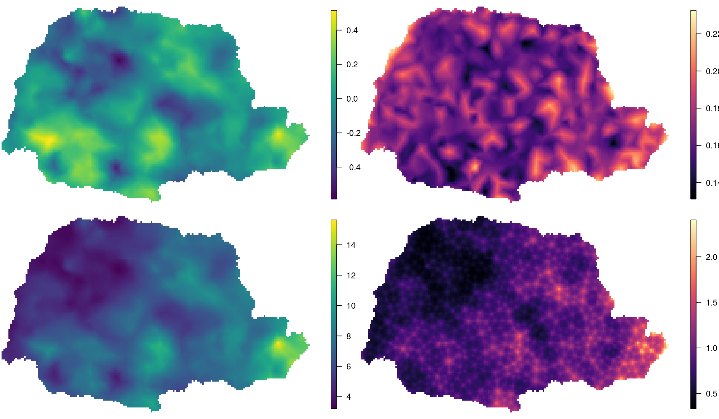
Figure 2.24: Posterior mean and standard deviation of the random field (top left and top right, respectively). Posterior mean and standard deviation for the response (bottom left and bottom right, respectively).
The posterior mean for the expected rainfall in January 2011 was higher near the ocean (to the east) and lower in the north-west side of Paraná state. Since the linear effect from the distance to the ocean will drive this pattern, the spatial effect in this case will account for deviations from this pattern. That is, the spatial effect is higher near the ocean and will add up to the higher effect from distance to the ocean, so that locations near the coast will have a higher posterior mean. The spatial effect is also higher in a region in the west, causing the expected values to be higher than what would be predicted by the linear effect alone.
2.8.4.2 Sampling at mesh nodes and interpolating
When all the covariates are smooth over space, it makes sense to make the predictions at the mesh nodes, where the spatial effect is estimated, and then project onto the grid. However, if a covariate is not smooth over space this approach no longer makes sense. The advantage of this approach is that it is computationally cheaper than to compute the full posterior marginals as in the previous examples.
In this example the idea is to compute the distance to the ocean effect at the mesh nodes. Then, compute the linear predictor at the mesh nodes. By that, it is possible to predict the response at the mesh nodes and then to interpolate it.
The first step is to compute the enviromental covariate at the mesh nodes:
oceanDist.mesh <- apply(
  spDists(PRborder[1034:1078, ], mesh$loc[, 1:2], longlat = TRUE),
  2, min)
The method presented now is based on getting samples from the posterior distribution of the linear predictor at the mesh nodes. Then, these values are interpolated to the grid and the expected value computed in the response scale by applying the inverse of the link function. As this is done for each sample (from the posterior distribution), this approach can be used to compute any quantity of interest, such as, for example, the mean and standard error.
The first step is to build the data stack for the prediction on the mesh:
stk.mesh <- inla.stack(
  data = list(y = NA),
  A = list(1, 1),
  effects = list(s = 1:spde$n.spde,
    data.frame(Intercept = 1, oceanDist = oceanDist.mesh)),
  tag = 'mesh')

stk.b <- inla.stack(stk.dat, stk.mesh)
Next, the model is fitted again, and similar options to reduce the computations
as in the previous example are set. In this case, an extra option is set to
include in the output the precision matrix for each hyperparameter
configuration for sampling from the joint posterior. This option is
control.compute = list(config = TRUE).
Hence, the code to fit the model is now:
rm.oceanD.l <- inla(f.oceanD.l, family = 'Gamma',
  data = inla.stack.data(stk.b),
  control.predictor = list(A = inla.stack.A(stk.b),
    compute = TRUE, link = 1),
  quantiles = NULL,
  control.results = list(return.marginals.random = FALSE,
    return.marginals.predictor = FALSE),
  control.compute = list(config = TRUE)) # Needed to sample
Sampling from the posterior distribution using the fitted model is done
using function inla.posterior.sample(). In the next example 1000 samples
from the posterior will be obtained:
sampl <- inla.posterior.sample(n = 1000, result = rm.oceanD.l)We do need to collect the index for the linear predictor corresponding to the stack data of the prediction scenario and use it to extract the corresponding elements of the latent field of each sample.
id.prd.mesh <- inla.stack.index(stk.b, 'mesh')$data
pred.nodes <- exp(sapply(sampl, function(x)
  x$latent[id.prd.mesh]))
Note that this is a matrix with the following dimensions:
dim(pred.nodes)
## [1]  967 1000
Computing the mean and standard deviation over the samples and projecting it is now:
sd.prd.s <- matrix(NA, nxy[1], nxy[2])
m.prd.s <- matrix(NA, nxy[1], nxy[2])

m.prd.s[xy.in] <- drop(Aprd %*% rowMeans(pred.nodes))
sd.prd.s[xy.in] <- drop(Aprd %*% apply(pred.nodes, 1, sd))
Finally, it is possible to check that this approach produces similar values as in the previous example (based on the computation of the posterior marginal):
cor(as.vector(m.prd.s), as.vector(m.prd), use = 'p')
## [1] 0.9998
cor(log(as.vector(sd.prd.s)), log(as.vector(sd.prd)), use = 'p')
## [1] 0.9605
References
Abrahamsen, P. 1997. “A Review of Gaussian Random Fields and Correlation Functions.” Norwegian Computing Center report No. 917.
Baddeley, A., E. Rubak, and R. Turner. 2015. Spatial Point Patterns: Methodology and Applications with R. Boca Raton, FL: Chapman & Hall/CRC.
Bakka, Haakon. 2018. “How to Solve the Stochastic Partial Differential Equation That Gives a Matérn Random Field Using the Finite Element Method.” arXiv Preprint arXiv:1803.03765.
Bakka, H., H. Rue, G.-A. Fuglstad, A. Riebler, D. Bolin, E. Krainski, D. Simpson, and F. Lindgren. 2018. “Spatial Modelling with R-INLA: A Review.” WIREs Comput Stat 10 (6): 1–24. https://doi.org/10.1002/wics.1443.
Banerjee, S., B. P. Carlin, and A. E. Gelfand. 2014. Hierarchical Modeling and Analysis for Spatial Data. 2nd ed. Boca Raton, FL: Chapman & Hall/CRC.
Besag, J. 1981. “On a System of Two-Dimensional Recurrence Equations.” J. R. Statist. Soc. B 43 (3): 302–9.
Bivand, R., T. Keitt, and B. Rowlingson. 2017. Rgdal: Bindings for the ’Geospatial’ Data Abstraction Library. https://CRAN.R-project.org/package=rgdal.
Bivand, R., J. Nowosad, and R. Lovelace. 2018. SpData: Datasets for Spatial Analysis. https://CRAN.R-project.org/package=spData.
Bivand, R., and G. Piras. 2015. “Comparing Implementations of Estimation Methods for Spatial Econometrics.” Journal of Statistical Software 63 (18): 1–36. https://www.jstatsoft.org/v63/i18/.
Bivand, R., and C. Rundel. 2017. Rgeos: Interface to Geometry Engine - Open Source (’Geos’). https://CRAN.R-project.org/package=rgeos.
Bivand, R. S., E. J. Pebesma, and V. Gomez-Rubio. 2013. Applied Spatial Data Analysis with R. 2nd ed. Springer, NY. http://www.asdar-book.org/.
Brenner, S. C., and R. Scott. 2007. The Mathematical Theory of Finite Element Methods. 3rd ed. Springer, New York.
Cameletti, M., F. Lindgren, D. Simpson, and H. Rue. 2013. “Spatio-Temporal Modeling of Particulate Matter Concentration Through the Spde Approach.” Advances in Statistical Analysis 97 (2): 109–31.
Chang, W., J. Cheng, J. J. Allaire, Y. Xie, and J. McPherson. 2018. Shiny: Web Application Framework for R. https://CRAN.R-project.org/package=shiny.
Ciarlet, P. G. 1978. The Finite Element Method for Elliptic Problems. Amsterdam: North-Holland.
Cressie, N. 1993. Statistics for Spatial Data. New York: Wiley.
Cressie, N., and C. K. Wikle. 2011. Statistics for Spatio-Temporal Data. Hoboken, NJ: John Wiley & Sons, Inc.
de Berg, M., O. Cheong, M. van Kreveld, and M. Overmars. 2008. Computational Geometry. 3rd ed. Berlin Heidelberg: Springer-Verlag.
Diggle, P. J. 2013. Statistical Analysis of Spatial and Spatio-Temporal Point Patterns. 3rd ed. Boca Raton, FL: Chapman & Hall/CRC Press.
Diggle, P. J., and P. J. Ribeiro Jr. 2007. Model-Based Geostatistics. Springer Series in Statistics. Hardcover.
Fuglstad, G-A., D. Simpson, F. Lindgren, and H. Rue. 2018. “Constructing Priors That Penalize the Complexity of Gaussian Random Fields.” Journal of the American Statistical Association to appear. https://doi.org/10.1080/01621459.2017.1415907.
Guibas, Leonidas J., D. E. Knuth, and M. Sharir. 1992. “Randomized Incremental Construction of Delaunay and Voronoi Diagrams.” Algorithmica 7 (1–6): 381–413.
Haining, R. 2003. Spatial Data Analysis: Theory and Practice. Cambridge University Press.
Illian, J., A. Penttinen, H. Stoyan, and D. Stoyan. 2008. Statistical Analysis and Modelling of Spatial Point Patterns. Chichester, UK: Wiley & Sons.
Lindgren, F. 2012. “Continuous Domain Spatial Models in R-INLA.” The ISBA Bulletin 19 (4): 14–20.
Lindgren, F., and H. Rue. 2015. “Bayesian Spatial and Spatio-Temporal Modelling with R-INLA.” Journal of Statistical Software 63 (19).
Lindgren, F., H. Rue, and J. Lindström. 2011. “An Explicit Link Between Gaussian Fields and Gaussian Markov Random Fields: The Stochastic Partial Differential Equation Approach (with Discussion).” J. R. Statist. Soc. B 73 (4): 423–98.
Pettit, L. I. 1990. “The Conditional Predictive Ordinate for the Normal Distribution.” Journal of the Royal Statistical Society: Series B (Methodological) 52 (1): 175–84.
Quarteroni, A. M., and A. Valli. 2008. Numerical Approximation of Partial Differential Equations. 2nd ed. New York: Springer.
Ribeiro Jr., P. J., and P. J. Diggle. 2001. “GeoR: A Package for Geostatistical Analysis.” R-NEWS 1 (2): 14–18. http://CRAN.R-project.org/doc/Rnews/.
Rowlingson, B., and P. Diggle. 2017. Splancs: Spatial and Space-Time Point Pattern Analysis. https://CRAN.R-project.org/package=splancs.
Rowlingson, B. S., and P. J. Diggle. 1993. “Splancs: Spatial Point Pattern Analysis Code in S-Plus.” Computers & Geosciences 19 (5): 627–55. https://doi.org/https://doi.org/10.1016/0098-3004(93)90099-Q.
Rozanov, J. A. 1977. “Markov Random Fields and Stochastic Partial Differential Equations.” Math. USSR Sbornik 32 (4)): 515–34. http://dx.doi.org/10.1070/SM1977v032n04ABEH002404.
Rue, H., and L. Held. 2005. Gaussian Markov Random Fields: Theory and Applications. Monographs on Statistics & Applied Probability. Boca Raton, FL: Chapman & Hall.
Rue, H., and H. Tjelmeland. 2002. “Fitting Gaussian Markov Random Fields to Gaussian Fields.” Scandinavian Journal of Statistics 29 (1): 31–49.
Schabenberger, O., and C. A. Gotway. 2004. Statistical Methods for Spatial Data Analysis. Boca Raton, FL: Chapman & Hall/CRC.
Simpson, D. P., H. Rue, A. Riebler, T. G. Martins, and S. H. Sørbye. 2017. “Penalising Model Component Complexity: A Principled, Practical Approach to Constructing Priors.” Statistical Science 32 (1): 1–28.
Sørbye, S., and H. Rue. 2014. “Scaling Intrinsic Gaussian Markov Random Field Priors in Spatial Modelling.” Spatial Statistics 8: 39–51.
Tobler, W. R. 1970. “A Computer Movie Simulating Urban Growth in the Detroid Region.” Economic Geography 2 (46): 234–40.