Chapter 5 Spatial non-stationarity
In this chapter we focus on non-stationary models. In particular, these models will show how to model the covariance using covariates and how to deal with physical barriers in the study region.
5.1 Explanatory variables in the covariance
In this section we present an example of the model proposed in Ingebrigtsen, Lindgren, and Steinsland (2014). This example describes a way to include explanatory variables (i.e., covariates) in both of the SPDE model parameters. We will consider the parametrization used along this book and detailed in Lindgren, Rue, and Lindström (2011).
5.1.1 Introduction
First of all, we remind ourselves of the definition for the precision matrix. Restricting to \(\alpha=1\) and \(\alpha=2\), the precision matrix is given as follows:
\(\alpha=1\): \(\mathbf{Q}_{1,\tau,\kappa} = \tau(\kappa^2\mathbf{C} + \mathbf{G})\)
\(\alpha=2\): \(\mathbf{Q}_{2,\tau,\kappa} = \tau(\kappa^4\mathbf{C} + \kappa^2\mathbf{G} + \kappa^2\mathbf{G} + \mathbf{G}\mathbf{C}^{-1}\mathbf{G})\)
The default stationary SPDE model implemented in inla.spde2.matern()
function considers the \(\theta_1\) as the log of the local precision parameter \(\tau\)
and \(\theta_2\) the log of the scale \(\kappa\) parameter.
The marginal variance \(\sigma^2\) and the range \(\rho\) are function of these parameters as
\(\sigma^2=\Gamma(\nu) / (\Gamma(\alpha)(4\pi)^{d/2}\kappa^{2\nu}\tau^2)\) and \(\rho = \sqrt{8\nu}/\kappa\). These relations give
\[\begin{align} \begin{array}{rcl} \log(\tau) & = & \frac{1}{2}\log\left(\frac{\Gamma(\nu)}{\Gamma(\alpha)(4\pi)^{d/2}}\right) - \log(\sigma) -\nu\log(\kappa) \\ \log(\kappa) & = & \frac{\log(8\nu)}{2} - \log(\rho). \end{array} \end{align}\]
The approach to non-stationarity proposed in Ingebrigtsen, Lindgren, and Steinsland (2014) is to consider a regression like model for \(\log\tau\) and \(\log\kappa\). It is done considering basis functions as
\[\begin{align}\begin{array}{rcl} \log(\tau(\mathbf{s})) & = & b_0^{(\tau)}(\mathbf{s}) + \sum_{k=1}^p b_k^{(\tau)}(\mathbf{s})\theta_k \\ \log(\kappa(\mathbf{s})) & = & b_0^{(\kappa)}(\mathbf{s}) + \sum_{k=1}^p b_k^{(\kappa)}(\mathbf{s})\theta_k \end{array}\end{align}\]
where we have the \(\theta_k\) parameters as regression on the basis functions. Setting \(\mathbf{T}\) as a diagonal matrix with elements as \(\tau(\mathbf{s})\) and \(\mathbf{K}\) a diagonal matrix with elements as \(\kappa(\mathbf{s})\) we now have the precision matrix as
\(\alpha=1\): \(\mathbf{Q}_{1,\theta,\mathbf{B}^{(\tau)},\mathbf{B}^{(\kappa)}}\) = \(\mathbf{T}(\mathbf{K}\mathbf{C}\mathbf{K} + \mathbf{G})\mathbf{T}\)
\(\alpha=2\): \(\mathbf{Q}_{2,\theta,\mathbf{B}^{(\tau)},\mathbf{B}^{(\kappa)}}\) = \(\mathbf{T}(\mathbf{K}^2\mathbf{C}\mathbf{K}^2 + \mathbf{K}\mathbf{G} + \mathbf{G}^T\mathbf{K} + \mathbf{G}\mathbf{C}^{-1}\mathbf{G})\mathbf{T}\)
These basis functions are passed in the argument B.tau and B.kappa
arguments of the inla.spde2.matern() function.
\(b_0^{(\tau)}\) goes in the first column of B.tau and \(b_k^{(\tau)}\) in the next columns.
\(b_0^{(\kappa)}\) goes in the first column of B.kappa and \(b_k^{(\tau)}\) in the next columns.
When these basis matrices are supplied as just one line matrix,
the actual basis matrix will be formed having all lines equal to this
unique line matrix and the model is stationary.
The default uses \([0\; 1\; 0]\) (one by three) matrix
for the local precision parameter \(\tau\) and \([0\; 0\; 1]\)
(one by three) matrix for the scaling parameter \(\kappa\).
Thus \(\theta_1\) controls \(\log(\tau)\) and \(\theta_2\) controls \(\log(\kappa)\).
We can use B.tau and B.kappa in such a way to build a
model for the marginal standard deviation and range, see Lindgren and Rue (2015).
This is the case of the function inla.spde2.pcmatern(), where
B.tau is \([\log(\tau_0) \; \nu \; -1]\) and
B.kappa is \([\log(\kappa_0) \; -1 \; 0]\).
We are using this along this book having the
range as the first parameter and \(\sigma\) the second.
Both the marginal standard deviation and the range can be modeled considering a regression model as detailed in Lindgren and Rue (2015). This is the case of considering that the log of \(\sigma\) and log of \(\rho\) are modeled by a regression on basis functions as
\[\begin{align} \log(\sigma(\mathbf{s})) = b_0^\sigma(\mathbf{s}) + \sum_{k=1}^p b_k^\sigma(\mathbf{s}) \theta_k \\ \log(\rho(\mathbf{s})) = b_0^{\rho}(\mathbf{s}) + \sum_{k=1}^p b_k^\rho(\mathbf{s}) \theta_k \end{align}\]
where \(b_0^\sigma(\mathbf{s})\) and \(b_0^{\rho(\mathbf{s})}\) are offsets,
\(b_k^\sigma()\) and \(b_k^{\rho()}\) are basis functions that can be defined on spatial
locations or covariates, each one with an associated \(\theta_k\) parameter.
Notice that B.tau and B.kappa are basis functions evaluated at each mesh
node. Therefore, to include a covariate in \(\sigma^2\) or in the range we do
need to have it available at each mesh node.
In our example we consider the domain area as the rectangle \((0,10)\times(0,5)\) and
the range as a function of the first coordinate of the location defined by
\(\rho(\mathbf{s}) = \exp(\theta_2 + \theta_3 (s_{i,1} - 5) / 10)\). This gives
\[\begin{align}\begin{array}{rcl} \log(\sigma) & = & \log(\sigma_0) + \theta_1 \\ \log(\rho(\mathbf{s})) & = & \log(\rho_0) + \theta_2 + \theta_3 b(\mathbf{s}) \end{array}\end{align}\]
where \(b(\mathbf{s}) = (s_{i,1}-5)/10\).
We now define the values for \(\theta_1\), \(\theta_2\) and \(\theta_3\). Because we choose \(\theta_3\) positive it implies an increasing range along the first location coordinate. The range as function of the first coordinate is shown in Figure 5.1.
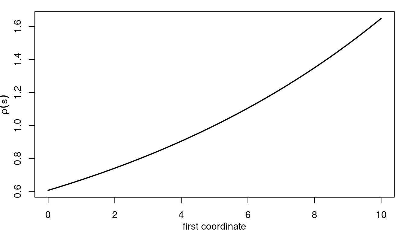
Figure 5.1: Range as function of the first coordinate.
We have to define the basis functions for \(\log(\tau)\) and \(\log(\kappa)\). Following Lindgren and Rue (2015) we need to write \(\log(\kappa(\mathbf{s}))\) and \(\log(\tau(\mathbf{s}))\) as functions of \(\log(\rho(\mathbf{s}))\) and \(\log(\sigma)\). Substituting \(\log(\sigma)\) and \(\log(\rho(\mathbf{s}))\) into the equations for \(\log(\kappa(\mathbf{s}))\) and \(\log(\tau(\mathbf{s}))\) we have
\[\begin{align}\begin{array}{rcl} \log(\tau(\mathbf{s})) & = & \log(\tau_0) - \theta_1 + \nu\theta_2 + \nu\theta_3 b(\mathbf{s}) \\ \log(\kappa(\mathbf{s})) & = & \log(\kappa_0) - \theta_2 - \theta_3 b(\mathbf{s}) \;. \end{array}\end{align}\]
Therefore we have to include \((s_{i,1}-5)/10\) as a fourth column in B.tau
and minus it in B.kappa as well.
5.1.2 Implementation of the model
First, we define the \((0,10)\times (0,5)\) rectangle:
pl01 <- cbind(c(0, 1, 1, 0, 0) * 10, c(0, 0, 1, 1, 0) * 5)The mesh will be created using this polygon, as follows:
mesh <- inla.mesh.2d(loc.domain = pl01, cutoff = 0.1,
  max.edge = c(0.3, 1), offset = c(0.5, 1.5))
This mesh is made of 2198 nodes.
We supply \((s_{i,1} - 5) / 10\) as a fourth column of in the B.tau argument of
the inla.spde2.matern() function, and minus it in the fourth column of
argument B.kappa. In addition, it is also necessary to set a prior
distribution on the vector of hyperparameters \(\theta\) according to its new
dimension, a three length vector. The default is a Gaussian distribution, for
which mean and precision diagonal need to be specified in two vectors, as
follows:
nu <- 1
alpha <- nu + 2 / 2
# log(kappa)
logkappa0 <- log(8 * nu) / 2
# log(tau); in two lines to keep code width within range
logtau0 <- (lgamma(nu) - lgamma(alpha) -1 * log(4 * pi)) / 2
logtau0 <- logtau0 - logkappa0
# SPDE model
spde <- inla.spde2.matern(mesh,
  B.tau = cbind(logtau0, -1, nu, nu * (mesh$loc[,1] - 5) / 10),
  B.kappa = cbind(logkappa0, 0, -1, -1 * (mesh$loc[,1] - 5) / 10),
  theta.prior.mean = rep(0, 3),
  theta.prior.prec = rep(1, 3))
The precision matrices are built with
Q <- inla.spde2.precision(spde, theta = theta)5.1.3 Simulation at the mesh nodes
We can draw one realization of the process using the inla.qsample() function as
sample <- as.vector(inla.qsample(1, Q, seed = 1))The top plot in Figure 5.2 shows the simulated values
projected to a grid Here, the projector matrix has been used to project the
simulated values in the grid limited in the unit square with limits (0, 10) and
(0, 5). The bottom plot in Figure 5.2 shows the spatial
correlation with respect to two points, computed using function
book.spatial.correlation(). The interesting issue to observe here is how
the range at which spatial autocorrelation disappears (i.e., correlation is
zero) is smaller around the point on the left due to the increasing range with
the x-coordinate simulated in the model.
The results and plots in Figure 5.2 have been computed with this code:
# Plot parameters
par(mfrow = c(2, 1), mar = c(0, 0, 0, 0))
#Plot Field
proj <- inla.mesh.projector(mesh, xlim = 0:1 * 10, ylim = 0:1 * 5,
  dims = c(200, 100))
book.plot.field(sample, projector = proj)
# Compute spatial autocorrelation
cx1y2.5 <- book.spatial.correlation(Q, c(1, 2.5), mesh)
cx7y2.5 <- book.spatial.correlation(Q, c(7, 2.5), mesh)
# Plot spatial autocorrelation
book.plot.field(cx1y2.5, projector = proj, zlim = c(0.1, 1))
book.plot.field(cx7y2.5, projector = proj, zlim = c(0.1, 1),
  add = TRUE)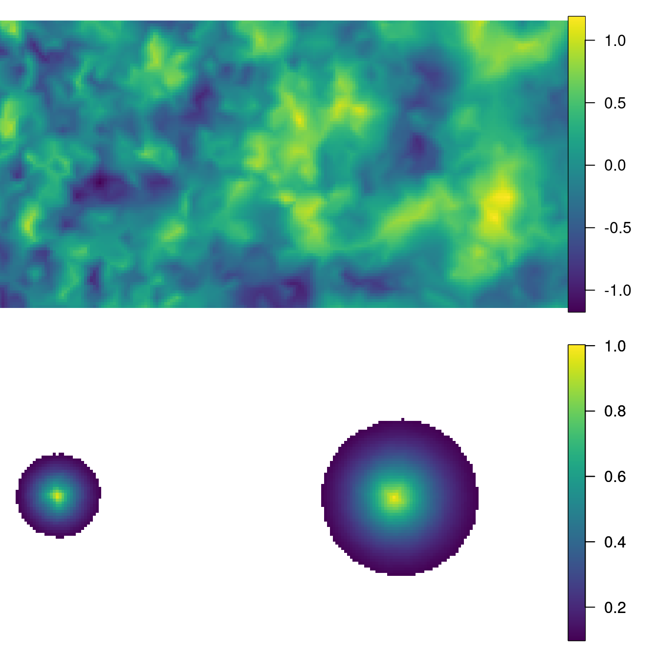
Figure 5.2: The simulated random field with increasing range along the horizontal coordinate (top) and the correlation at two location points: \((1,2.5)\) and \((7,2.5)\) (bottom).
5.1.4 Estimation with data simulated at the mesh nodes
A model can be easily fitted with the data simulated at mesh nodes. Considering that there are observations exactly at each mesh node, there is no need to use any predictor matrix and the stack functionality. Because data are just realizations from the random field, there is no noise and then the precision of the Gaussian likelihood will be fixed to a very large value. For example, to value \(\exp(20)\):
clik <- list(hyper = list(prec = list(initial = 20,
  fixed = TRUE)))
Because the random field has a zero mean, there are not fixed parameters to fit. Hence, model fitting can be done as follows:
formula <- y ~ 0 + f(i, model = spde)

res1 <- inla(formula, control.family = clik,
  data = data.frame(y = sample, i = 1:mesh$n))
Now, the summary of the posterior marginal distribution for \(\theta\) (joined with the true values) is provided in Table 5.1. The results obtained are quite good and the point estimates are very close to the actual values.
| Parameter | True | Mean | St. Dev. | 2.5% quant. | 97.5% quant. |
|---|---|---|---|---|---|
| \(\theta_1\) | -1 | -0.9800 | 0.0328 | -1.0413 | -0.9125 |
| \(\theta_2\) | 0 | 0.0006 | 0.0408 | -0.0749 | 0.0851 |
| \(\theta_3\) | 1 | 1.1679 | 0.0591 | 1.0530 | 1.2846 |
5.1.5 Estimation with locations not at the mesh nodes
The more general case is when observations are not at the mesh nodes.
For this reason, some in the next example data will be at the locations
simulated with the following R code:
set.seed(2)
n <- 200
loc <- cbind(runif(n) * 10, runif(n) * 5)
Next, we take the simulated random field at the mesh vertices and project it into these locations. For this, a projector matrix is needed:
projloc <- inla.mesh.projector(mesh, loc)Hence, the projection is:
x <- inla.mesh.project(projloc, sample)This provides the sample data at the simulated locations.
Now, because these locations are not vertices of the mesh, the stack functionality is required to put all the data together. First, the predictor matrix is needed, but this is the same used to sample the data.
Then, a stack is defined for this sample:
stk <- inla.stack(
  data = list(y = x),
  A = list(projloc$proj$A),
  effects = list(data.frame(i = 1:mesh$n)),
  tag = 'd')
Finally, the model is fitted:
res2 <- inla(formula, data = inla.stack.data(stk),
  control.family = clik,
  control.predictor = list(compute = TRUE, A = inla.stack.A(stk)))
The true values and a summary of marginal posterior distributions for \(\theta\) are given in Table 5.2. As in the previous example, estimates are quite close to the actual values of the parameters used in the simulation.
| Parameter | True | Mean | St. Dev. | 2.5% quant. | 97.5% quant. |
|---|---|---|---|---|---|
| \(\theta_1\) | -1 | -0.9115 | 0.0708 | -1.0507 | -0.7723 |
| \(\theta_2\) | 0 | -0.0063 | 0.1248 | -0.2539 | 0.2364 |
| \(\theta_3\) | 1 | 1.0367 | 0.2539 | 0.5547 | 1.5582 |
Figure 5.3 shows the simulated values, the predicted (posterior mean) and the projected posterior standard deviation. Here, it can be seen how the predicted values are similar to the simulated true values.
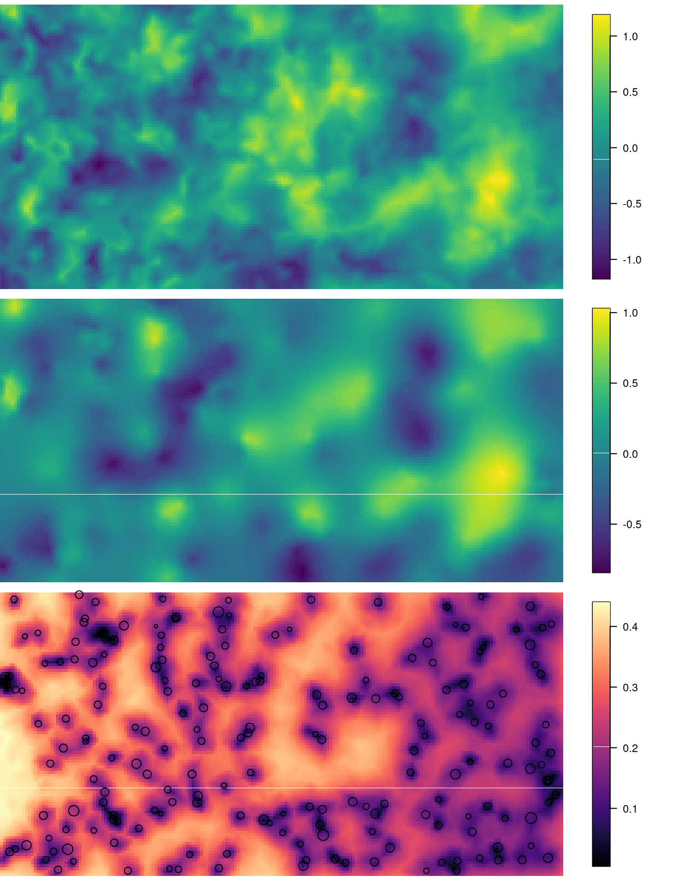
Figure 5.3: Simulated field (top), posterior mean (mid) and posterior standard deviation with the location points added (bottom).
5.2 The Barrier model
The most common spatial models are the stationary isotropic ones. For these, moving or rotating the map does not change the model. Even though this is a reasonable assumption in many cases, it is not a reasonable assumption if there are physical barriers in the study area. For example, when we model aquatic species near the coast, a stationary model cannot be aware of the coastline, and a new model is needed (one which is aware of the coastline).
In the paper by Bakka et al. (2016) a new non-stationary model was constructed for
use in INLA, with a syntax very similar to the stationary model (to make it
easy to use). In this section we give an example using this model on a part of
the Canadian coastline.
5.2.1 Canadian coastline example
The example developed here is based on simulated data using the Canadian coastline as a physical barrier to spatial correlation. This example requires some manipulation of maps and polygons in order to create an appropriate mesh for the model, and we have loaded additional packages for this.
5.2.1.1 Polygon
First, we construct some spatial polygon covering our study area. Here we do
this via the mapdata package (Becker, Wilks, and Brownrigg 2016):
# Select region
map <- map("world", "Canada", fill = TRUE,
  col = "transparent", plot = FALSE)
IDs <- sapply(strsplit(map$names, ":"), function(x) x[1])
map.sp <- map2SpatialPolygons(
  map, IDs = IDs,
  proj4string = CRS("+proj=longlat +datum=WGS84"))
Next, we define our study area pl.sel, as a manually constructed polygon, and
intersect this with the coastal area. Since we have a polygon for land, we
take the difference instead of an intersection, as follows:
pl.sel <- SpatialPolygons(list(Polygons(list(Polygon(
  cbind(c(-69, -62.2, -57, -57, -69, -69),
    c(47.8, 45.2, 49.2, 52, 52, 48)),
     FALSE)), '0')), proj4string = CRS(proj4string(map.sp)))

poly.water <- gDifference(pl.sel, map.sp)
The Canadian coastline and the manually constructed polygon can be seen on the left plot in Figure 5.4.
5.2.1.2 Transforming to UTM coordinates
So far we have used longitude and latitude in this example, but this is not a valid coordinate system for spatial modeling, as distances in longitude and distances in latitude are in different scales. Modeling should be done in a CRS (Coordinate Reference System) where units along each axis is measured in e.g. kilometers. We do not want to use meters as this would result in very large values along the axes, and could cause unstable numerical results.
The projection is done with function spTransform() as follows:
# Define UTM projection
kmproj <- CRS("+proj=utm +zone=20 ellps=WGS84 +units=km")
# Project data
poly.water = spTransform(poly.water, kmproj)
pl.sel = spTransform(pl.sel, kmproj)
map.sp = spTransform(map.sp, kmproj)
5.2.1.3 Simple mesh
Before we construct the mesh we are going to use, we first show how to construct a mesh only in water. We then discuss the difference between the two approaches.
mesh.not <- inla.mesh.2d(boundary = poly.water, max.edge = 30,
  cutoff = 2)
The created mesh has 1115 nodes. This mesh has been plotted in Figure 5.4 (right plot).
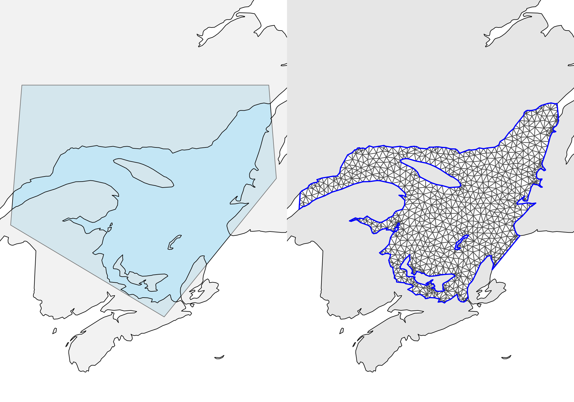
Figure 5.4: The left plot shows the polygon for land in grey and the manually constructed polygon for our study area in light blue. The right plot shows the simple mesh, constructed only in the water.
Before developing the Barrier model, we used to construct this simple mesh and use the SPDE model here, as this avoids smoothing across land. The problem with this approach, however, is that we introduce other hidden assumptions, called Neumann boundary conditions. As shown by Bakka et al. (2016), this assumption can lead to even worse behavior than the stationary model (which smooths over islands).
5.2.1.4 Mesh over land and sea
Next, we construct a mesh over both water and land. This is the mesh we are going to use. We include the coastline polygon in the function call, to make the edges of the triangles follow the coastline.
max.edge = 30
bound.outer = 150
mesh <- inla.mesh.2d(boundary = poly.water,
  max.edge = c(1,5) * max.edge,
  cutoff = 2,
  offset = c(max.edge, bound.outer))
Next, we select the triangles of the mesh that are inside poly.water. We
define the triangles in the barrier area (i.e. on land) to be all the triangles
that are not on water. From this we construct the poly.barrier. This should
match the original land polygon closely, but will deviate a little. The new
polygon poly.barrier is where our model assumes there to be land; hence we
use this polygon also for plotting the results.
water.tri = inla.over_sp_mesh(poly.water, y = mesh,
  type = "centroid", ignore.CRS = TRUE)
num.tri = length(mesh$graph$tv[, 1])
barrier.tri = setdiff(1:num.tri, water.tri)
poly.barrier = inla.barrier.polygon(mesh,
  barrier.triangles = barrier.tri)
The mesh in Figure 5.5 is different from the simple mesh in Figure 5.4, as we have also defined the mesh over land. We can use this mesh to construct both a stationary model and a Barrier model.
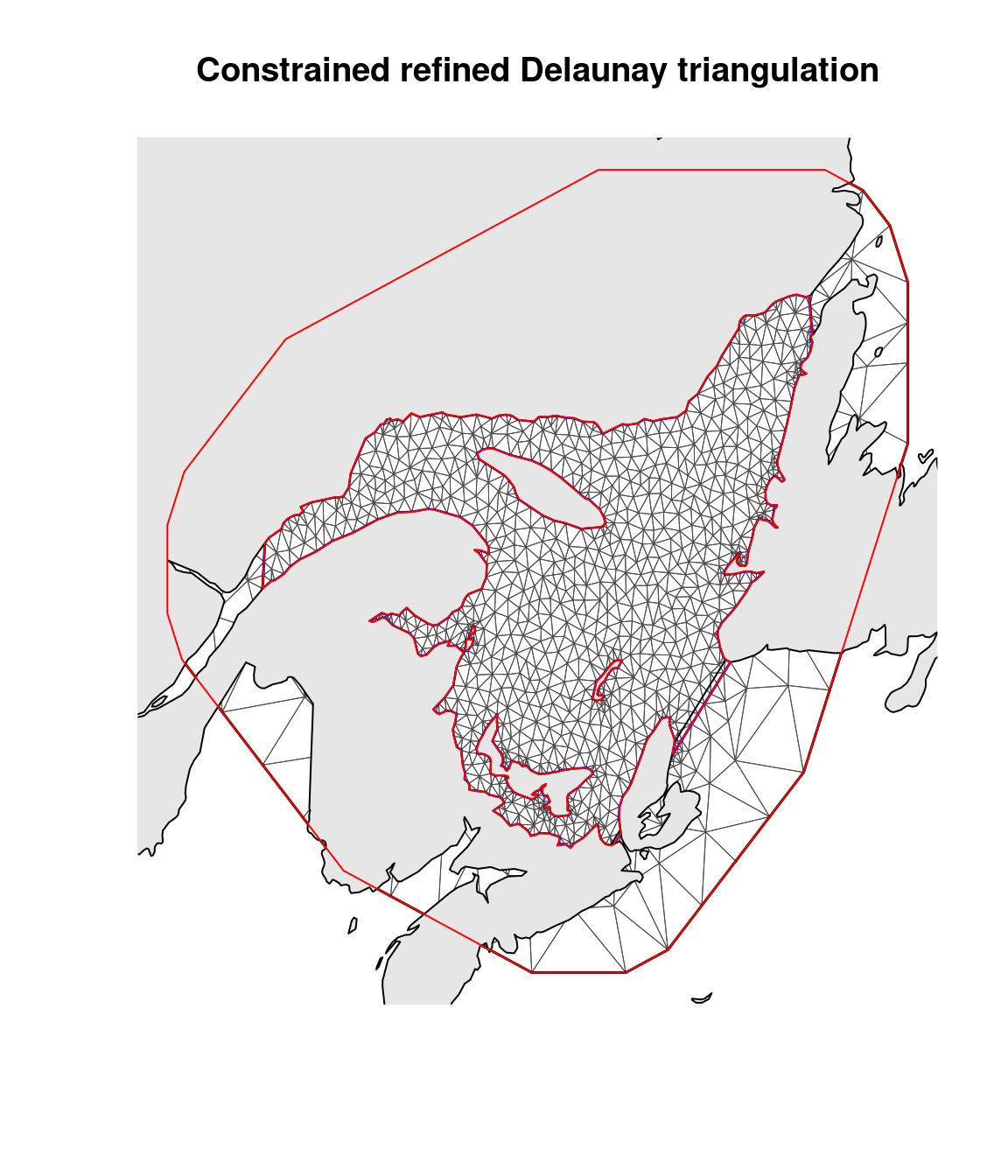
Figure 5.5: The mesh constructed both over water and land. The grey region is the original land map. The inner red outline marks the coastline barrier.
5.2.1.5 The Barrier model vs. the stationary model
Next we define the precision matrix for the Barrier model and the stationary model
\[ \mathbf{u} \sim \mathcal N(0, Q^{-1}) \] considering unit marginal variance:
range <- 200
barrier.model <- inla.barrier.pcmatern(mesh,
  barrier.triangles = barrier.tri)
Q <- inla.rgeneric.q(barrier.model, "Q", theta = c(0, log(range)))
This code spits out a warning because the priors are not defined. However, as we are simulating from the GF, the priors for the hyperparameters are irrelevant.
stationary.model <- inla.spde2.pcmatern(mesh,
  prior.range = c(1, 0.1), prior.sigma = c(1, 0.1))
Q.stat <- inla.spde2.precision(stationary.model,
  theta = c(log(range), 0))
The priors we chose here are arbitrary as they are not used. Note that the
ordering of theta is reversed between the two models.
We use the functions from spde-book-functions.R to compute spatial
correlation surfaces; see Figure 5.6.
# The location we find the correlation with respect to
loc.corr <- c(500, 5420)
corr <- book.spatial.correlation(Q, loc = loc.corr, mesh)
corr.stat <- book.spatial.correlation(Q.stat, loc = loc.corr,
  mesh)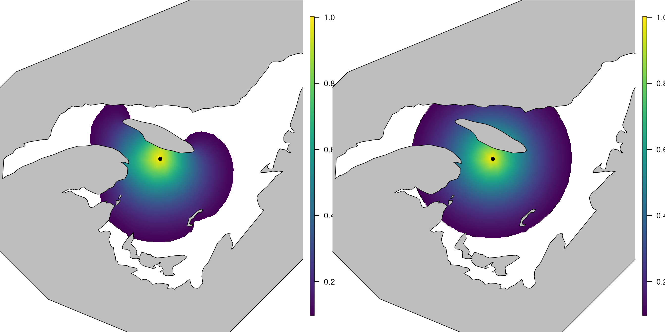
Figure 5.6: The left plot shows the correlation structure of the Barrier model, with respect to the black point, while the right plot shows the correlation structure of the stationary model.
5.2.1.6 Sample from the Barrier model
Next, we sample locations from the water polygon using spsample(). And we
simplify the data structure loc.data from SpatialPoints to just a matrix of
values.
set.seed(201805)
loc.data <- spsample(poly.water, n = 1000, type = "random")
loc.data <- loc.data@coords
We sample the continuous field \(\mathbf{u}\) and project it to data locations:
# Seed is the month the code was first written times some number
u <- inla.qsample(n = 1, Q = Q, seed = 201805 * 3)[, 1]
A.data <- inla.spde.make.A(mesh, loc.data)
u.data <- A.data %*% u

# df is the dataframe used for modeling
df <- data.frame(loc.data)
names(df) <- c('locx', 'locy')
# Size of the spatial signal
sigma.u <- 1
# Size of the measurement noise
sigma.epsilon <- 0.1
df$y <- drop(sigma.u * u.data + sigma.epsilon * rnorm(nrow(df)))
5.2.1.7 Inference with the Barrier model
Similarly as with previous models, we construct the typical stack object to prepare the data for model fitting:
stk <- inla.stack(
  data = list(y = df$y),
  A = list(A.data, 1),
  effects =list(s = 1:mesh$n, intercept = rep(1, nrow(df))),
  tag = 'est')
The formula for the model only takes an intercept plus the spatial effect:
form.barrier <- y ~ 0 + intercept + f(s, model = barrier.model)Finally, we run INLA with a Gaussian likelihood:
res.barrier <- inla(form.barrier, data = inla.stack.data(stk),
  control.predictor = list(A = inla.stack.A(stk)),
  family = 'gaussian',
  control.inla = list(int.strategy = "eb"))
5.2.1.8 Posterior spatial field
In Figure 5.7 we compare the results from the Barrier model to the true (simulated) spatial field. These have a close match. We observe quick changes across islands or small peninsulas, which may be smoothed out by a stationary model. See Bakka et al. (2016) for a more detailed discussion.
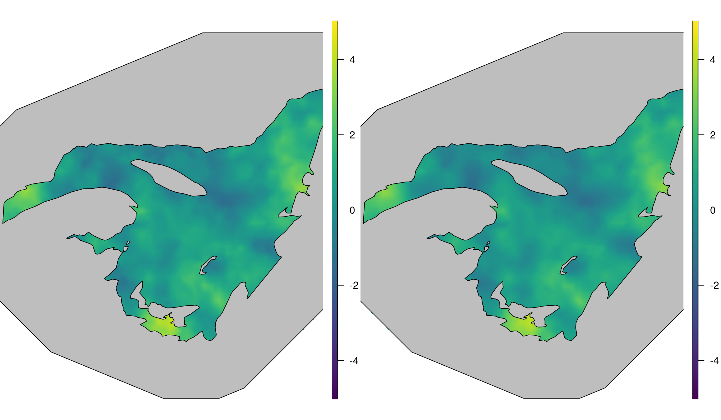
Figure 5.7: The left plot shows the true simulated spatial field \(\mathbf{u}\), while the right plot shows the posterior mean of the Barrier model.
5.2.1.9 Posterior of hyperparameters
The summary of the posterior marginals of the model hyperparameters is:
res.barrier$summary.hyperpar
##                                            mean     sd
## Precision for the Gaussian observations 94.4892 6.5776
## Theta1 for s                            -0.1348 0.1182
## Theta2 for s                             5.1357 0.1379
##                                         0.025quant 0.5quant
## Precision for the Gaussian observations    82.0188  94.3386
## Theta1 for s                               -0.3381  -0.1457
## Theta2 for s                                4.8992   5.1229
##                                         0.975quant    mode
## Precision for the Gaussian observations   107.8866 94.1400
## Theta1 for s                                0.1218 -0.1861
## Theta2 for s                                5.4352  5.0749
To summarize or plot the hyperparameters in the Barrier model, we must know the order they come in and the transformations:
\[\begin{align} \sigma &= e^ {\theta_1} \quad \text{is the marginal standard deviation} \\ r &= e^ {\theta_2} \quad \text{is the spatial range} \end{align}\]
From this we compute Table 5.3. We see that our estimates and intervals recover the true values.
| Parameter | True | 50% quant. | 2.5% quant. | 97.5% quant. |
|---|---|---|---|---|
| \(\sigma\) | 1 | 0.8644 | 0.7131 | 1.129 |
| \(range\) | 200 | 167.8143 | 134.1823 | 229.344 |
5.3 Barrier model for noise data in Albacete (Spain)
Barrier models can be appropriate tools to model different types of environmental phenomena that have a clear anisotropic behavior. A clear example is the propagation of noise in cities, where buildings act as barriers in the propagation of noise. In this section, spatial and spatio-temporal models are developed using noise data from the city of Albacete (Castilla-La Mancha, Spain).
Data has been extracted from a report commissioned by the local authorities due to increasing concern about noise in the city and, in particular, in certain areas of the city center. The analysis will focus on a busy area in the city center (popularly known as “La zona”, i.e., “The zone”) with plenty of bars and restaurants. The original reports are available (as PDF documents) from website http://www.pioneraconsultores.com/es/mapa-de-ruidos.zhtm?corp=medioambiente, which contains the original data.
Measurements were taken in March 2010 for a period of 24 hours at different points throughout the city. In this analysis, hourly measurements of sound pressure levels (in A-weighted decibels, or dbA) at 7 different points within the study region will be considered. Local regulations require noise levels to be below 65 db during the day and below 60 db at night in residential areas. Hence, the aim of this example is to study how noise levels vary within the city center to get an idea of whether local regulations are fulfilled.
The data used in this example is provided as a
SpatialPointsDataFrame in file noise.RData. Table 5.4
summarizes the main variables in the dataset.
| Variable | Description |
|---|---|
X |
x-coordinate (in UTM). |
Y |
y-coordinate (in UTM). |
LAeqZZh |
Hourly sound pressure level (in dbA) between ZZ and ZZ + 1 hours. ZZ is an integer from 1 to 24. |
5.3.0.1 Data loading
Data about the locations of the buildings, which will act as barriers, will be
obtained from OpenStreetMap (OSM, OpenStreetMap contributors 2018) using package osmar
(Eugster and Schlesinger 2013). This package provides a simple way to download OSM data and
extract the relevant information required to build the desired models.
In the next lines of R code, function osmsource_api() sets up access to
the OSM API. Next, function center_bbox is used to set the squared region
where the data is extracted from. The first two arguments are the coordinates
of the center of the rectangle, and the next two its width and height.
Finally, function get_osm() gets the data from the defined bounding box using
the OSM API.
#Get building data from Albacete using OpenStreetMap
library(osmar)

src <- osmsource_api()

bb <- center_bbox(-1.853152, 38.993318,  400, 400)
ua <- get_osm(bb, source = src)
OSM data provides a wealth of information about street data in variable ua.
Since our focus is on modeling noise using buildings as barriers, the
information about buildings will be extracted. Functions find() and
find_down() are used below to obtain an index of all features in the OSM data
in ua tagged as building. Then subset() is used to select the elements in
ua that are in the index of buildings. Finally, function as_sp converts the
boundaries of the buildings (as associated information) into a
SpatialPolygonsDataFrame.
idx <- find(ua, way(tags(k == "building")))
idx <- find_down(ua, way(idx))
bg <- subset(ua, ids = idx)

bg_poly <- as_sp(bg, "polygons")
The newly created SpatialPolygonsDataFrame object stores different buildings
as separate entities. Hence, we will use function unionSpatialPolygons() to
create a single entity, which will be used later to obtain the boundaries of
the streets.
library(maptools)
bg_poly <- unionSpatialPolygons(bg_poly,
  rep("1", length(bg_poly)))
Next, the actual study area is defined by using function center_bbox()
again, this time with a smaller width and height, to make sure that all
buildings in the study area have been retrieved before. Finally,
a SpatialPolygons object is created and the intersection between
the boundary of the study area and the polygons of the buildings is
created using function gIntersection from the rgeos package (R. Bivand and Rundel 2017).
#Outer boundary to overlay with buildings
bb.outer <- center_bbox(-1.853152, 38.993318,  350, 350)
pl <- matrix(c(bb.outer[1:2], bb.outer[c(3, 2)], bb.outer[3:4],
  bb.outer[c(1, 4)]), ncol = 2, byrow = TRUE)

pl_sp <- SpatialPolygons(
  list(Polygons(list(Polygon(pl)), ID = 1)),
  proj4string = CRS(proj4string(bg_poly)))

library(rgeos)

bg_poly2 <- gIntersection(bg_poly, pl_sp, byid = TRUE)
Coordinates of the buildings are in longitude and latitude, which is not
an adequate coordinate reference system to deal with distances. For this
reason, coordinates will be converted into UTM, so that distances
are measured in meters. For this, function spTransform() will be
used:
## Transform data
library(rgdal)
pl_sp.utm30 <- spTransform(pl_sp,
  CRS("+proj=utm +zone=30 +ellps=GRS80 +units=m +no_defs"))
bg_poly2.utm30 <- spTransform(bg_poly2,
  CRS("+proj=utm +zone=30 +ellps=GRS80 +units=m +no_defs"))
The last part of the building data processing involves obtaining not the polygons of the buildings, but the polygons of the streets, which is where the spatial process takes place. This will be done by taking the bounding box of the study region and removing the buildings, as follows:
## Compute difference to get streets
bg_poly2.utm30 <- gDifference(pl_sp.utm30, bg_poly2.utm30)
Figure 5.8 shows the buildings (left plot) and the streets (right plot) that will be used in the analysis.
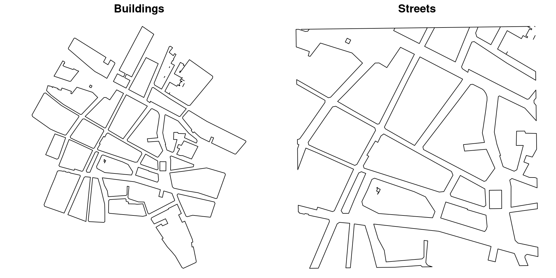
Figure 5.8: Building and street boundaries obtained from OpenStreetMap.
Noise data is provided in a data.frame in file noise.RData, and it
can be loaded as:
load("data/noise.RData")This dataset contains data from 7 locations where noise has been measured. This includes 5 outdoors locations plus 2 indoors locations. Although noise may be attenuated at these 2 locations they have been kept in the dataset to have more observations in the analysis.
5.3.0.2 Mesh building
The mesh will be built similarly to that in Section 5.2.1. In this case, distances are measured in meters. The maximum edges of the triangles will be 5 meters and the outer boundary will be 10 meters:
max.edge = 5
bound.outer = 10
mesh <- inla.mesh.2d(boundary = pl_sp.utm30,
  max.edge = c(1, 1.5) * max.edge,
  cutoff = 10,
  offset = c(max.edge, bound.outer))
The next lines of R code will use function inla.over_sp_mesh() (to
check which mesh triangles are inside a polygon) and call function
inla.barrier.polygon() to obtain the polygon around the barrier. Figure
5.9 shows the mesh created, together with the streets and the
polygon around the barrier obtained with inla.barrier.polygon() (in red).
city.tri = inla.over_sp_mesh(bg_poly2.utm30, y = mesh,
  type = "centroid", ignore.CRS = TRUE)
num.tri <- length(mesh$graph$tv[, 1])
barrier.tri <- setdiff(1:num.tri, city.tri)
poly.barrier <- inla.barrier.polygon(mesh,
  barrier.triangles = barrier.tri)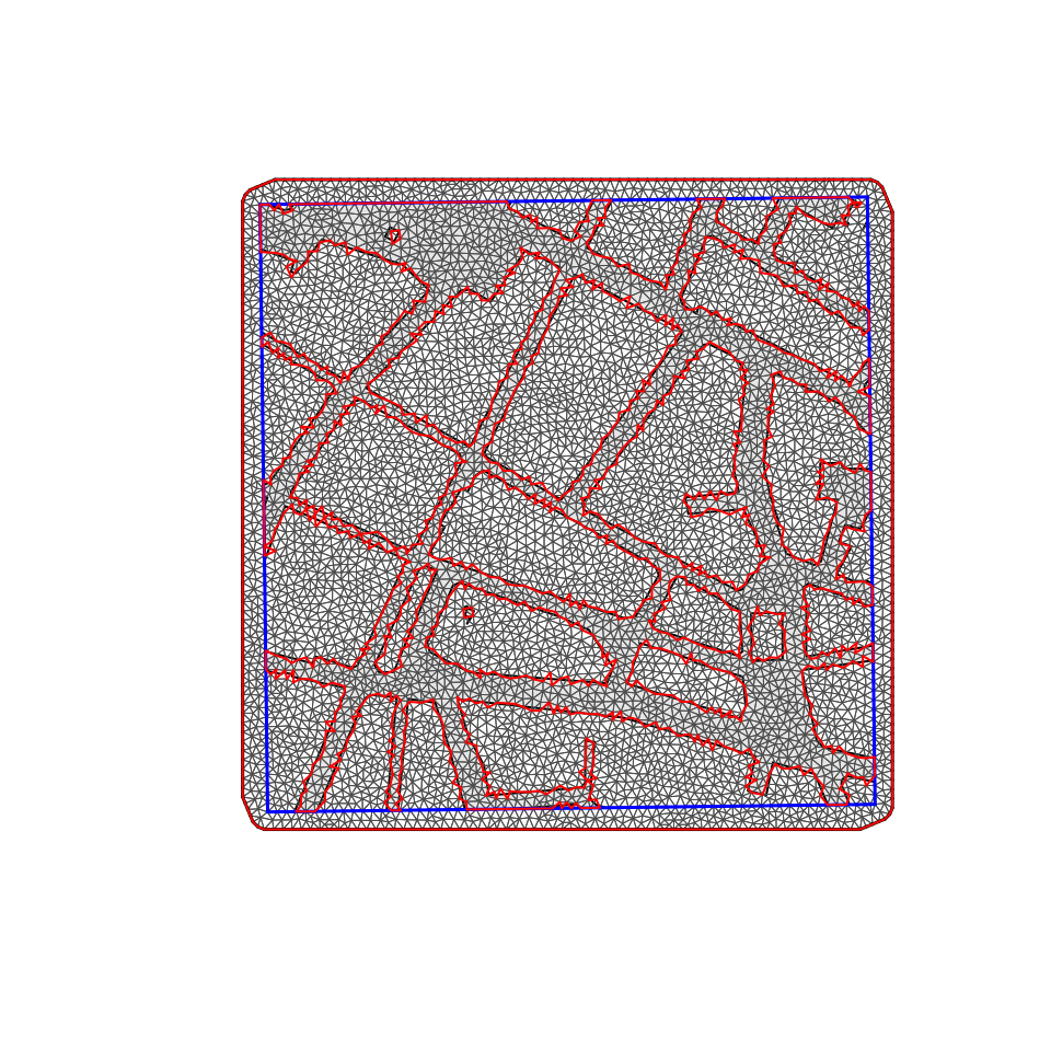
Figure 5.9: Mesh created for the analysis of noise data in Albacete (Spain).
5.3.0.3 Barrier model for noise data
Before fitting the actual barrier model to the noise data, we will explore how
the spatial correlation in the barrier model is defined. First of all, a model
with range 100 and precision 1 is simulated. Here, function
inla.barrier.pcmatern() is used to define a barrier model using the
rgeneric approach in INLA to define latent models; see
inla.doc("rgeneric") for details. Furthermore, inla.rgeneric.q() returns
the precision matrix of the model for some values of the hyperparameters, i.e.,
precision and range (in the log scale).
range <- 100
prec <- 1
barrier.model <- inla.barrier.pcmatern(mesh,
  barrier.triangles = barrier.tri)
Q <- inla.rgeneric.q(barrier.model, "Q",
  theta = c(log(prec), log(range)))
In order to compare the Barrier model, a stationary model is defined below.
Function inla.spde2.pcmatern() defines a stationary model using a PC prior
for the standard deviation and range, and function inla.spde2.precision()
returns the precision matrix of the model.
stationary.model <- inla.spde2.pcmatern(mesh,
  prior.range = c(100, 0.9), prior.sigma = c(1, 0.1))
Q.stat <- inla.spde2.precision(stationary.model,
  theta = c(log(range), 0))
Then, the correlation field at point (599318.3, 4316661) is computed
for the Barrier and stationary models:
# The location we find the correlation with respect to
loc.corr <- c(599318.3, 4316661)

corr <- book.spatial.correlation(Q, loc = loc.corr, mesh)
corr.stat = book.spatial.correlation(Q.stat, loc = loc.corr, mesh)
These are shown in Figure 5.10. Note how the spatial correlation for the stationary model (right plot in Figure 5.10) seems to ignore buildings and only considers Euclidean distance between two points, while the spatial autocorrelation for the Barrier model (left plot in Figure 5.10) does take buildings into account.
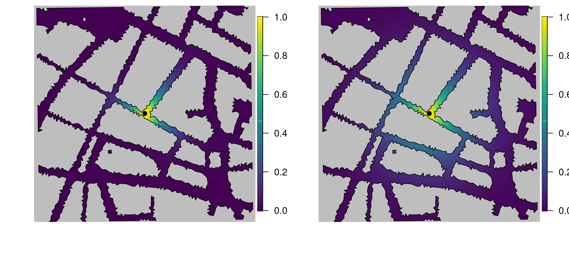
Figure 5.10: The left plot shows the correlation structure of the Barrier model, with respect to the black point, while the right plot shows the correlation structure of the stationary model.
The first Barrier model will consider the spatial variation of noise
at 1 am, which is measured by variable LAeq1h. The projector matrix
and stack required to fit the model can be obtained as follows:
A.data <- inla.spde.make.A(mesh, coordinates(noise))

stk <- inla.stack(
  data = list(y = noise$LAeq1h),
  A = list(A.data, 1),
  effects =list(s = 1:mesh$n, intercept = rep(1, nrow(noise))),
  tag = 'est')
Similarly, a new stack will be created for prediction at the mesh nodes:
# Projector matrix at prediction points
A.pred <- inla.spde.make.A(mesh, mesh$loc[, 1:2])

#Stack for prediction at mesh nodes
stk.pred <- inla.stack(
  data = list(y = NA),
  A = list(A.pred, 1),
  effects =list(s = 1:mesh$n, intercept = rep(1, nrow(A.pred))),
  tag = 'pred')

# Joint stack for model fitting and prediction
joint.stk <- inla.stack(stk, stk.pred)
Next, the formula to fit the model is:
form.barrier <- y ~ 0 + intercept + f(s, model = barrier.model)Then, the model is fitted using a PC prior on the standard deviation parameter of the likelihood:
# PC-prior for st. dev.
stdev.pcprior <- list(prior = "pc.prec", param = c(2, 0.01))
# Model fitting
res.barrier <- inla(form.barrier,
  data = inla.stack.data(joint.stk),
  control.predictor = list(A = inla.stack.A(joint.stk),
    compute = TRUE),
  family = 'gaussian',
  control.inla = list(int.strategy = "eb"),
  control.family = list(hyper = list(prec = stdev.pcprior)),
  control.mode = list(theta = c(1.647, 1.193, 3.975)))
The summary of the fitted model is shown below. Figure 5.11 shows estimates of the posterior mean and 97.5% quantile of the noise. As can be seen, it is clear that noise level at 1 am seems to be very close to or higher than the cut off of 65 dB.
summary(res.barrier)
##
## Call:
##    c("inla(formula = form.barrier, family = \"gaussian\",
##    data = inla.stack.data(joint.stk), ", "
##    control.predictor = list(A = inla.stack.A(joint.stk),
##    compute = TRUE), ", " control.family = list(hyper =
##    list(prec = stdev.pcprior)), ", " control.inla =
##    list(int.strategy = \"eb\"), control.mode = list(theta
##    = c(1.647, ", " 1.193, 3.975)))")
## Time used:
##     Pre = 0.592, Running = 111, Post = 1.26, Total = 113
## Fixed effects:
##            mean    sd 0.025quant 0.5quant 0.975quant  mode kld
## intercept 64.89 1.389      62.17    64.89      67.62 64.89   0
##
## Random effects:
##   Name     Model
##     s RGeneric2
##
## Model hyperparameters:
##                                         mean    sd 0.025quant
## Precision for the Gaussian observations 5.46 0.701      4.211
## Theta1 for s                            1.04 0.145      0.731
## Theta2 for s                            4.25 0.861      2.712
##                                         0.5quant 0.975quant
## Precision for the Gaussian observations     5.42       6.96
## Theta1 for s                                1.05       1.29
## Theta2 for s                                4.18       6.03
##                                         mode
## Precision for the Gaussian observations 5.33
## Theta1 for s                            1.09
## Theta2 for s                            3.87
##
## Expected number of effective parameters(stdev): 6.92(0.00)
## Number of equivalent replicates : 1.01
##
## Marginal log-Likelihood:  -32.65
## Posterior marginals for the linear predictor and
##  the fitted values are computed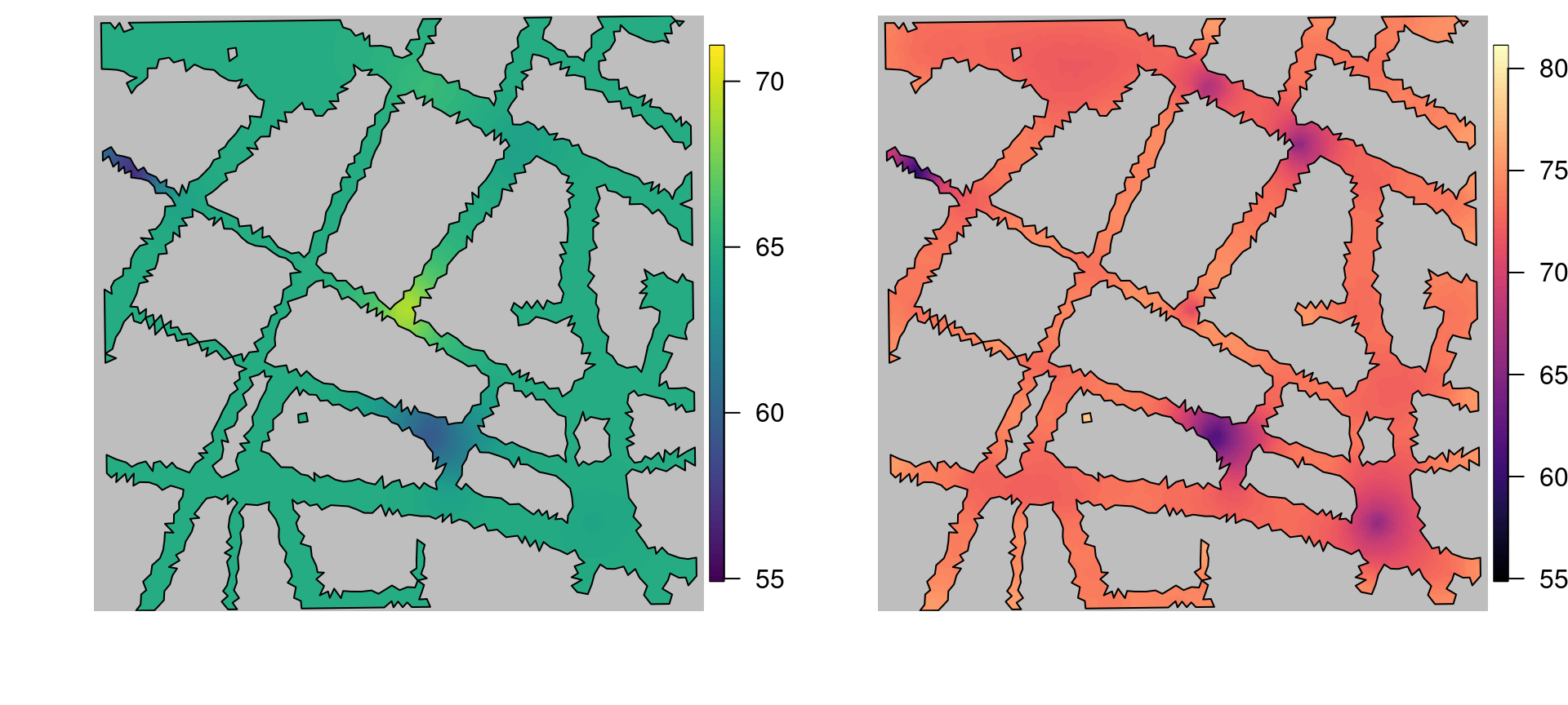
Figure 5.11: The left plot shows the posterior mean of the Barrier model, while the right plot shows the 97.5% quantile.
5.3.0.4 Space-time model
Space-time models are fully described in Chapter 7 and Chapter 8, but we have included here a simple example using the noise data. Given that information is available for 24 hours, it is possible to fit a space-time model to the noise data. First, a projector matrix is defined for the measurement points for the 24 hours:
A.st <- inla.spde.make.A(mesh = mesh,
  loc = coordinates(noise)[rep(1:7, 24), ])
The INLA stack is now created by adding variables LAeq1h, … LAeq24h
together with a time identifier (from 1 to 24 hours):
stk.st <- inla.stack(
  data = list(y = unlist(noise@data[, 2 + 1:24])),
  A = list(A.st, 1, 1),
  effects = list(s = 1:mesh$n,
    intercept = rep(1, 24 * nrow(noise)),
    time = rep(1:24, each = nrow(noise) )))
The model to be fitted is similar to the previous one, but now a cyclic random walk of order 1 is added as a separable time effect:
# Model formula
form.barrier.st <- y ~ 0 + intercept +
  f(s, model = barrier.model) +
  f(time, model = "rw1", cyclic = TRUE, scale.model = TRUE,
    hyper = list(prec = stdev.pcprior))
Note that a PC prior has been used on the standard deviation parameter of the random walk effect. Then the model is fitted similarly as before:
res.barrier.st <- inla(form.barrier.st,
  data = inla.stack.data(stk.st),
  control.predictor = list(A = inla.stack.A(stk.st)),
  family = 'gaussian',
  control.inla = list(int.strategy = "eb"),
  control.family = list(hyper = list(prec = stdev.pcprior)),
  control.mode = list(theta = c(-1.883, 1.123, 3.995, -0.837)))
A summary of the fitted model can be seen below. Figure 5.12 shows noise estimates at 6, 12, 18 and 24 hours.
summary(res.barrier.st)
##
## Call:
##    c("inla(formula = form.barrier.st, family =
##    \"gaussian\", data = inla.stack.data(stk.st), ", "
##    control.predictor = list(A = inla.stack.A(stk.st)),
##    control.family = list(hyper = list(prec =
##    stdev.pcprior)), ", " control.inla = list(int.strategy
##    = \"eb\"), control.mode = list(theta = c(-1.883, ", "
##    1.123, 3.995, -0.837)))")
## Time used:
##     Pre = 0.459, Running = 7.2, Post = 0.134, Total = 7.79
## Fixed effects:
##            mean    sd 0.025quant 0.5quant 0.975quant  mode kld
## intercept 64.86 1.468      61.98    64.86      67.74 64.86   0
##
## Random effects:
##   Name     Model
##     s RGeneric2
##    time RW1 model
##
## Model hyperparameters:
##                                          mean    sd 0.025quant
## Precision for the Gaussian observations 0.153 0.017      0.121
## Theta1 for s                            1.118 0.232      0.660
## Theta2 for s                            3.999 0.307      3.395
## Precision for time                      0.454 0.139      0.242
##                                         0.5quant 0.975quant
## Precision for the Gaussian observations    0.152      0.189
## Theta1 for s                               1.119      1.571
## Theta2 for s                               3.998      4.606
## Precision for time                         0.434      0.784
##                                          mode
## Precision for the Gaussian observations 0.150
## Theta1 for s                            1.123
## Theta2 for s                            3.995
## Precision for time                      0.397
##
## Expected number of effective parameters(stdev): 17.54(0.00)
## Number of equivalent replicates : 9.58
##
## Marginal log-Likelihood:  -452.70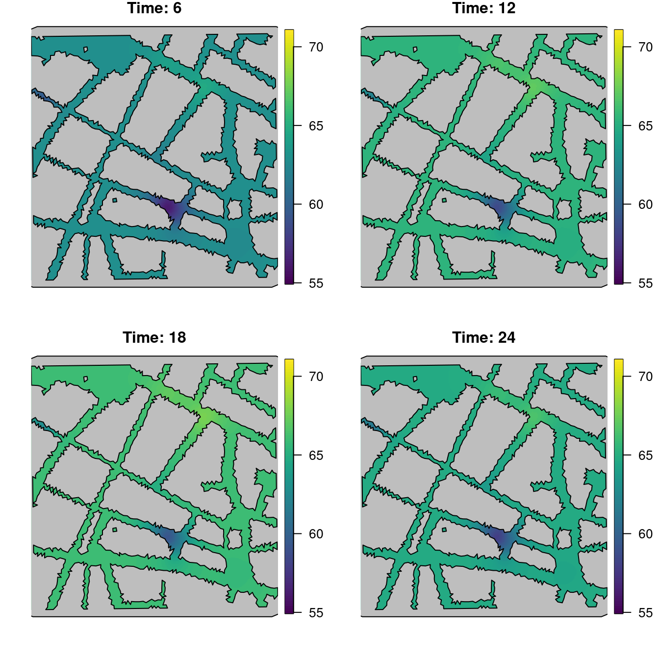
Figure 5.12: Point estimates of the noise level at different times.
References
Bakka, H., J. Vanhatalo, J. Illian, D. Simpson, and H. Rue. 2016. “Non-stationary Gaussian models with physical barriers.” ArXiv E-Prints, August. http://arxiv.org/abs/1608.03787.
Becker, R. A., A. R. Wilks, and R. Brownrigg. 2016. Mapdata: Extra Map Databases. https://CRAN.R-project.org/package=mapdata.
Bivand, R., and C. Rundel. 2017. Rgeos: Interface to Geometry Engine - Open Source (’Geos’). https://CRAN.R-project.org/package=rgeos.
Eugster, Manuel J. A., and Thomas Schlesinger. 2013. “Osmar: OpenStreetMap and R.” The R Journal 5 (1): 53–63. http://journal.r-project.org/archive/2013/RJ-2013-005/index.html.
Ingebrigtsen, R., F. Lindgren, and I. Steinsland. 2014. “Spatial Models with Explanatory Variables in the Dependence Structure.” Spatial Statistics 8: 20–38.
Lindgren, F., and H. Rue. 2015. “Bayesian Spatial and Spatio-Temporal Modelling with R-INLA.” Journal of Statistical Software 63 (19).
Lindgren, F., H. Rue, and J. Lindström. 2011. “An Explicit Link Between Gaussian Fields and Gaussian Markov Random Fields: The Stochastic Partial Differential Equation Approach (with Discussion).” J. R. Statist. Soc. B 73 (4): 423–98.
OpenStreetMap contributors. 2018. “Planet dump retrieved from https://planet.osm.org.” https://www.openstreetmap.org.