Chapter 6 Risk assessment using non-standard likelihoods

In this chapter we show how to use several different likelihoods that are related to risk assessment, combining them with the use of a spatial field.

The first example is about survival modeling where the outcome is the time to an event. This kind of outcome is common in medical studies where time to cure or time to death are common outcomes and in industry where time to failure is a common outcome. Most studies end before all of the patients are dead, or items have failed. In this case we use a censored likelihood; the likelihood considers the accumulated probability for the individual being alive until the study ends. We will only consider a simple case of censoring, but more complicated models are possible (see ?inla.surv).

In the second example we consider modeling extreme events. In this case the data is, usually, the maximum over several observations collected over time, for example, annual maxima of daily rainfall. The common likelihood will not fit these kind of data and thus specific ones are considered. In the example in this chapter, the Generalized Extreme Value (GEV) distribution and the Pareto Distribution (PD) are being considered. We consider the inference for blockwise maxima data and the inference for threshold exceedances cases in order to illustrate two approaches for modeling this kind of data.

6.1 Survival analysis

In this section we show how to fit a survival model using a continuous spatial random effect modeled through the SPDE approach. The example is based on the data presented in Henderson, Shimakura, and Gorst (2003). This data consists of 1043 cases of acute myeloid leukemia in adults recorded in New England between 1982 and 1998 by the North West Leukemia Register in the United Kingdom. The original code for the analysis is in Lindgren, Rue, and Lindström (2011) and it has been adapted here to use the stack functionality. In Section 6.1.1 how to fit a parametric survival model is considered, while in Section 6.1.2 we show how to fit the semiparametric Cox proportional hazard model.

6.1.1 Parametric survival model

The Leuk dataset records the 1043 cases, and includes residential location and other information about the patients. These are summarized in Table 6.1 and full details are provided in Henderson, Shimakura, and Gorst (2003).

Table 6.1: Description of the Leuk dataset on survival to acute myeloid leukemia (AML).

Variable	Description
time	Survival time (in days).
cens	Death/censorship indicator (1 = observed, 0 = censored).
xcoord	x-coordinate of residence.
ycoord	y-coordinate of residence.
age	Age of the patient.
sex	Sex of the patient (0 = female, 1 = male).
wbc	White blood cell count (WBC) at diagnosis, truncated at 500 units.
tpi	Measure of deprivation for the enumeration district of residence (higher values indicate less affluent areas).
district	District of residence.

This is included in INLA and can be loaded and summarized as follows:

data(Leuk)
# Survival time as year
Leuk$time <- Leuk$time / 365
round(sapply(Leuk[, c(1, 2, 5:8)], summary), 2)
##          time cens   age  sex    wbc   tpi
## Min.     0.00 0.00 14.00 0.00   0.00 -6.09
## 1st Qu.  0.11 1.00 49.00 0.00   1.80 -2.70
## Median   0.51 1.00 65.00 1.00   7.90 -0.37
## Mean     1.46 0.84 60.73 0.52  38.59  0.34
## 3rd Qu.  1.47 1.00 74.00 1.00  38.65  2.93
## Max.    13.64 1.00 92.00 1.00 500.00  9.55

The reason we measure time in years instead of days is to standardize the input for inla(). The likelihood for survival data has the exp(y * a) as its expression, where a is a model parameter and y is the response. Thus, we must be careful not to input too large or too small values, or the algorithm may face numerical instabilities.

The Kaplan-Meyer maximum likelihood estimates of the survival curve by sex with the respective 95% confidence interval has been computed and visualized in Figure 6.1 with:

library(survival)
km <- survfit(Surv(time, cens) ~ sex, Leuk) 
par(mar = c(2.5, 2.5, 0.5, 0.5), mgp = c(1.5, 0.5, 0), las = 1)
plot(km, conf.int = TRUE, col = 2:1) 
legend('topright', c('female', 'male'), lty = 1, col = 2:1,
  bty = "n")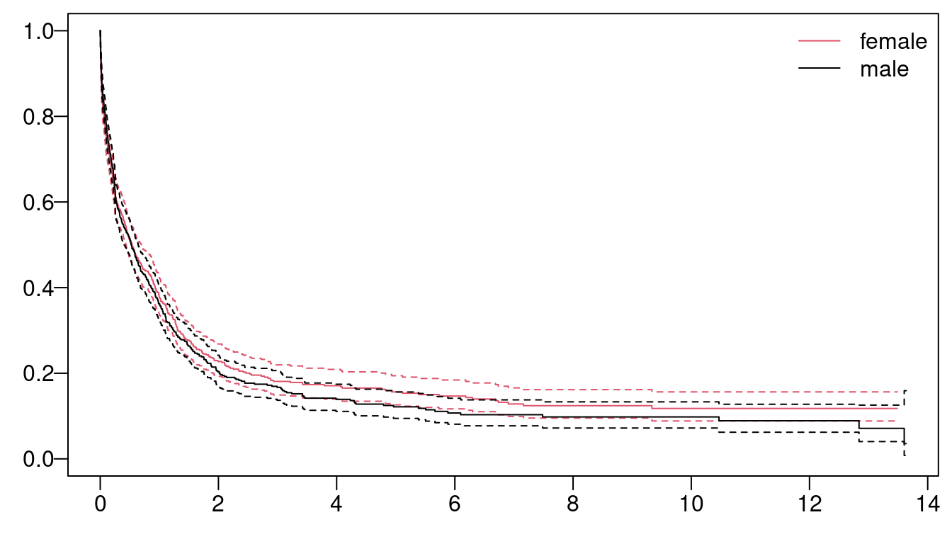 

Figure 6.1: Survival time as function of gender.

The mesh for the SPDE model is built taking into account the coordinates available in the dataset, using the following code:

loc <- cbind(Leuk$xcoord, Leuk$ycoord)
nwseg <- inla.sp2segment(nwEngland)

bnd1 <- inla.nonconvex.hull(nwseg$loc, 0.03, 0.1, resol = 50)
bnd2 <- inla.nonconvex.hull(nwseg$loc, 0.25)
mesh <- inla.mesh.2d(loc, boundary = list(bnd1, bnd2),
  max.edge = c(0.05, 0.2), cutoff = 0.02)

Next, the projector matrix is obtained with:

A <- inla.spde.make.A(mesh, loc)

For the parameters of the SPDE model, namely the practical range and the marginal standard deviation, we will consider the PC-prior derived in Fuglstad et al. (2018), defined as:

spde <- inla.spde2.pcmatern(mesh = mesh,
  prior.range = c(0.05, 0.01), # P(range < 0.05) = 0.01
  prior.sigma = c(1, 0.01)) # P(sigma > 1) = 0.01

In this example, a weibullsurv likelihood is considered. However, other parametric likelihoods can be used as well; for example, up to date we have in INLA: loglogistic, lognormal, exponential and weibullcure. The Weibull distribution in INLA has two variants, see inla.doc("weibull"), and the default has a mean equal to \(\Gamma(1+1/\alpha)\exp{(-\alpha\eta)}\), where \(\alpha\) is a shape parameter and \(\eta\) is the linear predictor. Thus, the expected value is inversely proportional to the linear predictor, whereas the survival is directly proportional.

The formula for the linear predictor, including the intercept and covariates is

form0 <- inla.surv(time, cens) ~ 0 + a0 + sex + age + wbc + tpi 

and adding the SPDE model is

form <- update(form0, . ~ . + f(spatial, model = spde))

Note how the formula includes a term using function inla.surv() to handle the observed time and the censoring status typical in survival data. This is common when working with survival outcomes due to the need to add the censoring information together with the survival time. The trick for building the data stack is to include all the variables needed in the formula. For the response these are time and the censoring status cens. The variables needed to define the spatial effect, namely the intercept and the covariates, are included as in previous models.

stk <- inla.stack(
  data = list(time = Leuk$time, cens = Leuk$cens), 
  A = list(A, 1), 
  effect = list(
    list(spatial = 1:spde$n.spde), 
    data.frame(a0 = 1, Leuk[, -c(1:4)]))) 

Next, we will fit the model considering this data stack.

r <- inla(
  form, family = "weibullsurv", data = inla.stack.data(stk), 
  control.predictor = list(A = inla.stack.A(stk), compute = TRUE)) 

Summary statistics of the posterior distribution of the intercept and the covariate effects can be extracted with the following code. Since we did not standardize the covariates, the effect sizes are not comparable.

round(r$summary.fixed, 4)
##        mean     sd 0.025quant 0.5quant 0.975quant    mode kld
## a0  -2.1700 0.2089    -2.5774  -2.1721    -1.7466 -2.1739   0
## sex  0.0718 0.0692    -0.0641   0.0717     0.2076  0.0717   0
## age  0.0327 0.0022     0.0284   0.0327     0.0371  0.0327   0
## wbc  0.0031 0.0005     0.0021   0.0031     0.0039  0.0031   0
## tpi  0.0245 0.0098     0.0051   0.0245     0.0437  0.0245   0

Similarly, summary statistics from the posterior distribution of the hyperparameters can be obtained as follows:

round(r$summary.hyperpar, 4)
##                                   mean     sd 0.025quant
## alpha parameter for weibullsurv 0.5991 0.0161     0.5681
## Range for spatial               0.3313 0.1659     0.1251
## Stdev for spatial               0.2937 0.0745     0.1738
##                                 0.5quant 0.975quant   mode
## alpha parameter for weibullsurv   0.5989     0.6314 0.5984
## Range for spatial                 0.2933     0.7580 0.2343
## Stdev for spatial                 0.2848     0.4651 0.2681

The spatial effect can be represented in a map. The polygons of each district in New England is also loaded when loading Leuk. First, a projection from the mesh into a grid is defined considering the bounding box around New England:

bbnw <- bbox(nwEngland)
r0 <- diff(range(bbnw[1, ])) / diff(range(bbnw[2, ]))
prj <- inla.mesh.projector(mesh, xlim = bbnw[1, ], 
  ylim = bbnw[2, ], dims = c(200 * r0, 200))

Then, the spatial effect (i.e., posterior mean and standard deviation) is interpolated and NA values are assigned to all the grid points that are outside of the region of interest:

spat.m <- inla.mesh.project(prj, r$summary.random$spatial$mean)
spat.sd <- inla.mesh.project(prj, r$summary.random$spatial$sd)
ov <- over(SpatialPoints(prj$lattice$loc), nwEngland)
spat.sd[is.na(ov)] <- NA
spat.m[is.na(ov)] <- NA

The posterior mean and standard deviation are displayed in Figure 6.2. As a result, the spatial effect has continuous variation along the region, rather than being constant inside each district.

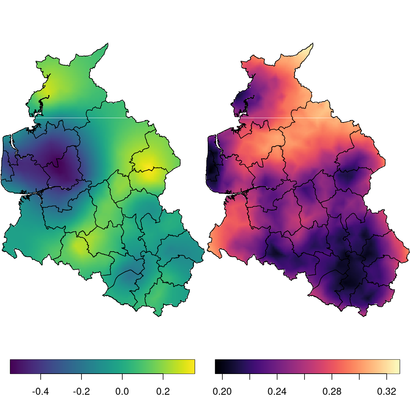
Figure 6.2: Map of the spatial effect for the Weibull survival model. Posterior mean (left) and posterior standard deviation (right).

6.1.2 Cox proportional hazard survival model

The Cox proportional hazard survival model (coxph family in INLA) is very common and we can fit it using maximum likelihood with the coxph() function from the survival package (Therneau 2015; Therneau and Grambsch 2000), with:

m0 <- coxph(Surv(time, cens) ~ sex + age + wbc + tpi, Leuk)

This model can be written as a Poisson regression. This idea was proposed in Holford (1980), detailed in Laird and Olivier (1981) and studied in Andersen and Gill (1982). In INLA we can prepare survival data for fitting a Cox proportional hazard model using the Poisson likelihood using the inla.coxph() function (Martino, Akerkar, and Rue 2010). We supply in this function a formula without the spatial effect, just to have the data prepared for fitting the Cox proportional hazard survival model as a Poisson model. The output from the inla.coxph() function will be supplied in the inla.stack() function together with the spatial terms.

cph.leuk <- inla.coxph(form0,
  data = data.frame(a0 = 1, Leuk[, 1:8]),
  control.hazard = list(n.intervals = 25))

For comparison purposes, we fit the model without the spatial effect considering the coxph family in INLA:

cph.res0 <- inla(form0, family = 'coxph', 
  data = data.frame(a0 = 1, Leuk[, c(1,2, 5:8)])) 

The next code changes the original formula updating it on the output and we will use it to add the spatial effect:

cph.formula <- update(cph.leuk$formula, 
  '. ~ . + f(spatial, model = spde)')

The projector matrix can be built as follows:

cph.A <- inla.spde.make.A(mesh,
  loc = cbind(cph.leuk$data$xcoord, cph.leuk$data$ycoord))

Finally, the data stack is built considering the relevant data from the output from the inla.coxph() function:

cph.stk <- inla.stack(
  data = c(list(E = cph.leuk$E), cph.leuk$data[c('y..coxph')]),
  A = list(cph.A, 1),
  effects = list(
    list(spatial = 1:spde$n.spde), 
      cph.leuk$data[c('baseline.hazard', 'a0', 
        'age', 'sex', 'wbc', 'tpi')]))

cph.data <- c(inla.stack.data(cph.stk), cph.leuk$data.list)

Then, the model is fitted considering a Poisson likelihood:

cph.res <- inla(cph.formula, family = 'Poisson', 
  data = cph.data, E = cph.data$E, 
  control.predictor = list(A = inla.stack.A(cph.stk)))

We now compare the estimated fixed effects from these results:

round(data.frame(surv = coef(summary(m0))[, c(1,3)], 
  r0 = cph.res0$summary.fixed[-1, 1:2], 
  r1 = cph.res$summary.fixed[-1, 1:2]), 4) 
##     surv.coef surv.se.coef. r0.mean  r0.sd r1.mean  r1.sd
## sex    0.0522        0.0678  0.0579 0.0679  0.0685 0.0692
## age    0.0296        0.0021  0.0333 0.0021  0.0348 0.0023
## wbc    0.0031        0.0004  0.0034 0.0005  0.0034 0.0005
## tpi    0.0293        0.0090  0.0342 0.0090  0.0322 0.0098

Regarding the spatial effects, the fitted values of the spatial effects are very similar between the two models fitted (Weibull and Cox):

s.m <- inla.mesh.project(prj, cph.res$summary.random$spatial$mean)
cor(as.vector(spat.m),  as.vector(s.m), use = 'p')
## [1] 0.9935
s.sd <- inla.mesh.project(prj, cph.res$summary.random$spatial$sd)
cor(log(as.vector(spat.sd)), log(as.vector(s.sd)), use = 'p')
## [1] 0.9987

6.2 Models for extremes

6.2.1 Motivation

Extreme Value Theory (EVT) emerges as the natural tool to assess probabilities of events that are rare, and whose occurrence involves great risk (Coles 2001). From the applied point of view, EVT provides a framework to develop techniques and models to address important problems related to risk assessment in many different areas, such as hydrology, wind engineering, climate change, flood monitoring and prediction, and large insurance claims.

When modeling extreme events, we typically need to extrapolate beyond observed data, into the tail of the distribution, where the available data are often limited, and classical inference methods usually fail. The plausibility of the extrapolation is subject to certain stability conditions that constrain the class of possible distributions on which extrapolation should be based.

In the context of univariate observations, EVT is based on an asymptotic characterization of maxima of a collection of independent and identically distributed (i.i.d.) random variables. Given i.i.d. continuous data \(Y_1,\ldots,Y_n\) and \(M_n = \max\{Y_1,\ldots,Y_n\}\), it can be shown that if the normalized distribution of \(M_n\) converges as \(n\to\infty\), then it converges to a Generalized Extreme-Value (GEV) distribution. The GEV is characterized by a location, a scale, and shape parameters (see, e.g., Coles 2001, Chapter 3). In practice, this asymptotic result serves as a justification to use the GEV distribution to model maxima over finite blocks of time, like monthly or annual maxima. Nevertheless, if the data are available at a finer resolution, then an alternative characterization of extremes might be given by the so-called threshold exceedances approach, where the interest is on observations that exceed a certain high predefined threshold. It can be shown that if the conditions for the GEV limit of normalized maxima hold, then as the threshold becomes large, the distribution of threshold exceedances converges to the generalized Pareto (GP) distribution characterized by a scale and shape parameters.

In practical applications, extreme observations are rarely independent. This has motivated the development of methodology to account for temporal non-stationarity in the distributions of interest. Typical approaches to this problem are based on the generalized linear modeling framework, allowing the parameters of a marginal distribution to depend on covariates (Davison and Smith 1990). Semi-parametric approaches for block maxima of bivariate vectors were introduced by Castro-Camilo and de Carvalho (2017) and Castro-Camilo, de Carvalho, and Wadsworth (2018). Hierarchical Bayesian models for threshold exceedances were introduced in Casson and Coles (1999), Cooley, Nychka, and Naveau (2007), and Opitz et al. (2018). Here we assume that GEV and GP observations are conditionally independent given a latent process that drives the spatial (or space-time) trends, as well as the dependence structure. In the following sections, we show how to simulate from and fit such models under the SPDE framework.

6.2.2 Simulating from the GEV and GP distributions

6.2.2.1 The random field and the linear predictor

We start by generating \(n=200\) random locations where we assume data are observed. These locations are also used as triangulation nodes to create the mesh:

library(INLA)
set.seed(1)
n <- 200
loc.data <- matrix(runif(n * 2), n, 2)
mesh <- inla.mesh.2d(loc = loc.data, cutoff = 0.05, 
  offset = c(0.1, 0.4), max.edge = c(0.05, 0.5))

The selected cutoff avoids creating too many small triangles. The SPDE model defined at the nodes of the mesh is constructed as follows:

spde <- inla.spde2.pcmatern(mesh,
  prior.range = c(0.5, 0.5),
  prior.sigma = c(0.5, 0.5))

Note that we use a PC-prior specification for the range and the marginal standard deviation. Specifically, we assume that \(\text{P}(\text{range} < 0.5) = 0.5\) and \(\text{P}(\text{std. dev} > 0.5) = 0.5\). We compute the precision matrix (Qu) for the true range (range) and marginal standard deviation (sigma.u) as follows:

sigma.u <- 2 
range <- 0.7 
Qu <- inla.spde.precision(spde,
  theta = c(log(range), log(sigma.u)))

Now we can generate \(m=40\) samples from the spatial field \(\mathbf{u}\):

m <- 40 # number of replications in time
set.seed(1)
u <- inla.qsample(n = m, Q = Qu, seed = 1)

The spatial field \(\mathbf{u}\) is a continuous simulation for the entire study area. To obtain simulations over the \(n\) random locations previously generated, we project \(\mathbf{u}\) over the locations:

A <- inla.spde.make.A(mesh = mesh, loc = loc.data)
u <- (A %*% u)

Note that the dimension of A is:

dim(A)
## [1] 200 461

This is the number of locations (\(n\)) times the number of nodes in the mesh (mesh$n). We are now able to define our linear predictor. For simplicity, we choose a linear predictor of the form \(\eta_i = \beta_0 + \beta_1 x + \mathbf{u}(\mathbf{s}_i)\), where \(x\) is a covariate and \(\mathbf{u}(\mathbf{s}_i)\) is the spatial field at location \(\mathbf{s}_i\):

b_0 <- 1 # intercept
b_1 <- 2 # coefficient for covariate
set.seed(1)
covariate <- rnorm(m*n)
lin.pred <- b_0 + b_1 * covariate + as.vector(u)

6.2.2.1.1 Samples from the GEV distribution

In INLA, the GEV distribution is parametrized in terms of a location parameter \(\mu\in\mathbb{R}\), a shape parameter \(\xi\in\mathbb{R}\), and a precision parameter \(\tau>0\):

\[\begin{equation} \label{eq:gev} G(y;\mu,\tau,\xi) = \exp\left\{-\left[1 + \xi\sqrt{\tau s}(y-\mu)\right]^{-1/\xi}\right\}, \quad\text{for } 1+\xi\sqrt{\tau s} (y-\mu)>0, \end{equation}\]

where \(s>0\) is a fixed scaling. The current implementation only allows the linear predictor to be linked to the location parameter using the identity link, i.e., \(\mu = \eta\). We generate \(m\times n\) samples from a GEV distribution using the rgev() function from the evd package (Stephenson 2002) as follows:

s <- 0.01
tau <- 4
s.y <- 1/sqrt(s*tau) # true scale
xi.gev <- 0.1 # true shape
library(evd)
set.seed(1)
y.gev <- rgev(n = length(lin.pred), loc = lin.pred, 
  shape = xi.gev, scale = s.y)

6.2.2.1.2 Samples from the GP distribution

The generalized Pareto distribution has a cumulative distribution function given by

\[\begin{equation*} G(y;\sigma,\xi) = 1 - \left(1 + \xi\frac{y}{\sigma}\right)^{-1/\xi},\quad y>0,\text{ } \xi \neq 0. \end{equation*}\]

Note that the exponential distribution arises in the limiting case, as for \(\xi\to 0\), we have \(G(y;\sigma) = 1-\exp(-y/\sigma)\). In INLA, the linear predictor controls the \(\alpha\)-quantile of the GP distribution:

\[\begin{align*} \text{P}{}(y\leq q_\alpha) &= \alpha,\\ q_\alpha &= \exp(\eta), \end{align*}\]

where \(\alpha\in(0,1)\) is provided by the user. The scale parameter \(\sigma\in\mathbb{R}\) is then a function of \(q_\alpha\) and \(\xi\): \[\begin{equation*} \sigma = \frac{\xi\exp(\eta)}{(1-\alpha)^{-\xi} - 1}. \end{equation*}\]

Using the probability integral transform, we can generate samples from the GP distribution by defining the following function:

rgp = function(n, sigma, eta, alpha, xi = 0.001){
  if (missing(sigma)) {
    stopifnot(!missing(eta) && !missing(alpha))
    sigma = exp(eta) * xi / ((1.0 - alpha)^(-xi) - 1.0)
  }
  return (sigma / xi * (runif(n)^(-xi) - 1.0))
}

Note that function rgp() is conveniently parametrized in terms of the scale \(\sigma\), the linear predictor \(\eta\), and the probability \(\alpha\) (i.e., the INLA parametrization). A sample of size \(m\times n\) from the GP can then be obtained as follows:

xi.gp <- 0.3
alpha <- 0.5 # median
q <- exp(lin.pred)
scale <- xi.gp * q / ((1 - alpha)^(-xi.gp) - 1)
set.seed(1)
y.gp <- rgp(length(lin.pred), sigma = scale, eta = lin.pred, 
  alpha = alpha, xi = xi.gp)

Note that in this case, the linear predictor is linked to the median of the distribution (since \(\alpha=0.5)\).

6.2.3 Inference for the GEV and GP distributions

6.2.3.1 Inference for blockwise maxima

We start by generating a new mesh and A matrix to fit our model:

mesh <- inla.mesh.2d(loc = loc.data, cutoff = 0.05, 
  max.edge = c(0.05, 0.1))
rep.id <- rep(1:m, each = n)
x.loc <- rep(loc.data[, 1], m)
y.loc <- rep(loc.data[, 2], m)
A <- inla.spde.make.A(mesh = mesh, loc = cbind(x.loc, y.loc), 
  group = rep.id)

Note that the dimension of the matrix A (8000, 24880) that we use for inference is much bigger that the one we used before. This is because we have \(m=40\) replications in time of a spatial field projected over \(n=200\) locations (\(n\times m = 8000\)), and the dimension of our new mesh is mesh$n = 624 (\(m \times\) mesh$n \(=24960\)).

We specify our prior model for the spatial effect, on the median of the parameters, as follows:

prior.median.sd <- 1
prior.median.range <- 0.7
spde <- inla.spde2.pcmatern(mesh, 
  prior.range = c(prior.median.range, 0.5), 
  prior.sigma = c(prior.median.sd, 0.5))

We obtain the named index vectors required for the SPDE model:

mesh.index <- inla.spde.make.index(name = "field", 
  n.spde = spde$n.spde, n.group = m)

We stack our data using the inla.stack() function:

stack <- inla.stack(
  data = list(y = y.gev), 
  A = list(A, 1, 1), 
  effects = list(mesh.index, 
    intercept = rep(1, length(lin.pred)), 
    covar = covariate),
  tag = "est")

Posterior marginals for the parameters of the GEV model are obtained by fitting the model with INLA. Here we use initial values to speed up inference (using variable init below). If you do not know what initial values to use, init can be set to NULL.

# Model formula
formula <- y ~ -1 + intercept + covar + 
  f(field, model = spde, group = field.group,
    control.group = list(model = "iid"))
# Initial values of hyperparameters
init = c(-3.253,  9.714, -0.503,  0.595)
# Prior on GEV parameters
hyper.gev = list(tail = list(prior = "gaussian", 
  param = c(0, 0.01), initial = log(1)))
# Mode fitting
res.gev <- inla(formula, 
  data = inla.stack.data(stack), 
  family ="gev",
  control.inla = list(strategy = "adaptive"),
  control.mode = list(restart = TRUE, theta = init),
  control.family = list(hyper = hyper.gev,
    gev.scale.xi = 0.01),
  control.predictor = list(A = inla.stack.A(stack), 
    compute = TRUE))

We specify model = 'iid' because we are assuming to have independent replicates in time. A summary for the model hyperparameters, i.e., the practical range and the marginal standard deviation for the latent Gaussian random field, along with the scale and shape parameters of the GEV can be obtained as:

tab.res.GEV <- round(cbind(true = c(1 / s.y^2, xi.gev, range,
    sigma.u),
  res.gev$summary.hyperpar), 4)

This summary is available in Table 6.2 together with the true values of the parameters used to simulate the data.

Table 6.2: Summary of the posterior distributions of the parameters and their true values.

Parameter	True	Mean	St. Dev.	2.5% quant.	97.5% quant.
Precision for GEV	0.04	0.0390	0.0009	0.0372	0.0408
Shape for GEV	0.10	0.0996	0.0080	0.0851	0.1165
Range for field	0.70	0.6038	0.0637	0.4856	0.7354
Stdev for field	2.00	1.9750	0.1006	1.7838	2.1796

6.2.3.2 Inference for threshold exceedances

The shape parameter \(\xi\in\mathbb{R}\) plays an important role in determining the weight of the upper tail: heavy tails are obtained with \(\xi >0\), light tails with \(\xi \to0\), and bounded tails with \(\xi < 0\). Moreover, if \(\xi \geq1\) then the mean is infinite, and if \(\xi\geq1/2\) then the variance is infinite. Therefore, for many practical applications, large values of \(\xi\) are unrealistic. Here we show how to specify this prior information using an approximation to the PC-prior for \(\xi\).

The current implementation for the GP distribution in INLA allows us to specify an Gamma prior distribution for \(\xi\) (or in the INLA parametrization, log-Gamma for \(\theta=\log(\xi)\)) that resembles a PC-prior for suitable choices of the Gamma shape and rate parameters. Specifically, Opitz et al. (2018) showed that the PC-prior for \(\xi\) when the simpler model is the exponential distribution (i.e. \(\xi=0\)) is

\[ \pi(\xi) = \tilde{\lambda}\exp\left\{-\tilde{\lambda}\frac{\xi}{(1-\xi)^{1/2}}\right\}\left\{\frac{1-\xi/2}{(1-\xi)^{3/2}}\right\}, \quad 0\leq\xi<1, \]

where \(\lambda = \tilde{\lambda}/\sqrt{2}\) is the penalization rate parameter (Fuglstad et al. 2018). The PC-prior \(\pi(\xi)\) can be approximated when \(\xi\to0\) by an exponential distribution with rate \(\tilde{\lambda}\) (or Gamma distribution with unit shape and rate \(\tilde{\lambda}\)):

\[ \tilde{\pi}(\xi) = \sqrt{2}\lambda\exp(-\sqrt{2}\lambda\xi) = \tilde{\lambda}\exp(-\tilde{\lambda}\xi),\quad \xi\geq 0. \]

Figure 6.3 shows that both priors are very similar to each other for large values of the penalization rate \(\lambda\), and differ for smaller values.

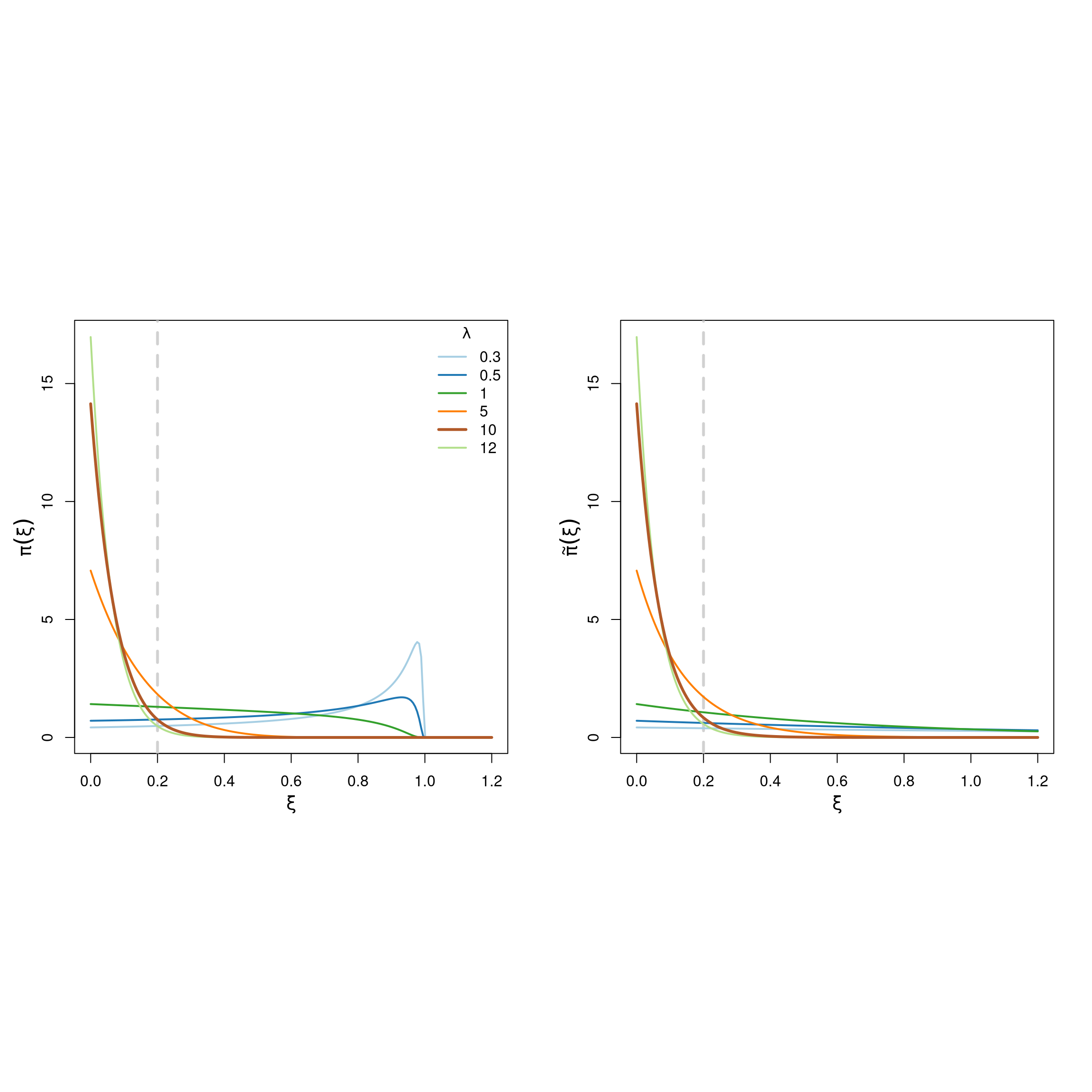
Figure 6.3: PC-priors for the GP shape parameter \(\xi\) for different values of the penalization rate \(\lambda\).

As mentioned before, we would like to specify a prior for \(\xi\) that drifts away from large values. To do this, we choose \(\lambda=10\), which implies that \(\text{P}(\xi > 0.2) = 0.06\) under \(\tilde{\pi}\) (see Figure 6.3). We specify this in the INLA framework as follows:

hyper.gp = list(tail = list(prior = "loggamma",
  param = c(1, 10)))

Using the SPDE model defined in Section 6.2.3.1, we fit our model for exceedances as follows:

# Data stack
stack <- inla.stack(
  data = list(y = y.gp),
  A = list(A, 1, 1),
  effects = list(mesh.index,
    intercept = rep(1, length(lin.pred)),
    covar = covariate),
  tag = "est")
#Initial values of the hyperparameters
init2 <- c(-1.3, -0.42, 0.62)
# Model fitting
res.gp <- inla(formula, 
  data = inla.stack.data(stack, spde = spde), 
  family ="gp",
  control.inla = list(strategy = "adaptive"),
  control.mode = list(restart = TRUE, theta = init2),
  control.family = list(list(control.link = list(quantile = 0.5),
    hyper = hyper.gp)),
  control.predictor = list(A = inla.stack.A(stack),
    compute = TRUE))

As with the GEV fit, the summary for the model hyperparameters can be obtained as:

table.results.GP <- round(cbind(true = c(xi.gp, range, sigma.u),
            res.gp$summary.hyperpar), 4)

This is available in Table 6.3, together with the true values of the parameters.

Table 6.3: Summary of the posterior distributions.

Parameter	True	Mean	St. Dev.	2.5% quant.	97.5% quant.
Shape for GP	0.3	0.2562	0.0183	0.2207	0.2926
Range for field	0.7	0.6646	0.0305	0.6078	0.7276
Stdev for field	2.0	1.9079	0.0619	1.7905	2.0336

References

Andersen, P. K., and R. D. Gill. 1982. “Cox’s Regression Model for Counting Processes: A Large Sample Study.” The Annals of Statistics 10 (4): 1100–1120.

Casson, E., and S. Coles. 1999. “Spatial Regression Models for Extremes.” Extremes 1 (4): 449–68.

Castro-Camilo, D., and M. de Carvalho. 2017. “Spectral Density Regression for Bivariate Extremes.” Stochastic Environmental Research and Risk Assessment 31 (7): 1603–13.

Castro-Camilo, D., M. de Carvalho, and J. Wadsworth. 2018. “Time-Varying Extreme Value Dependence with Application to Leading European Stock Markets.” Annals of Applied Statistics 12 (1): 283–309.

Coles, S. 2001. An Introduction to Statistical Modeling of Extreme Values. Vol. 208. London: Springer-Verlag.

Cooley, D., D. Nychka, and P. Naveau. 2007. “Bayesian Spatial Modeling of Extreme Precipitation Return Levels.” Journal of the American Statistical Association 102 (479): 824–40.

Davison, A. C., and R. L. Smith. 1990. “Models for Exceedances over High Thresholds (with Discussion).” Journal of the Royal Statistical Society: Series B, 393–442.

Fuglstad, G-A., D. Simpson, F. Lindgren, and H. Rue. 2018. “Constructing Priors That Penalize the Complexity of Gaussian Random Fields.” Journal of the American Statistical Association to appear. https://doi.org/10.1080/01621459.2017.1415907.

Henderson, R., S. Shimakura, and D. Gorst. 2003. “Modeling Spatial Variation in Leukemia Survival Data.” JASA 97 (460): 965–72.

Holford, T. R. 1980. “The Analysis of Rates and of Survivorship Using Log-Linear Models.” Biometrics 36: 299–305.

Laird, N., and D Olivier. 1981. “Covariance Analysis of Censored Survival Data Using Log-Linear Analysis Techniques.” Journal of the American Statistical Association 76: 231–40.

Lindgren, F., H. Rue, and J. Lindström. 2011. “An Explicit Link Between Gaussian Fields and Gaussian Markov Random Fields: The Stochastic Partial Differential Equation Approach (with Discussion).” J. R. Statist. Soc. B 73 (4): 423–98.

Martino, S., R. Akerkar, and H. Rue. 2010. “Approximate Bayesian Inference for Survival Models.” Scandinavian Journal of Statistics 28 (3): 514–28.

Opitz, T., R. Huser, H. Bakka, and H. Rue. 2018. “INLA Goes Extreme: Bayesian Tail Regression for the Estimation of High Spatio-Temporal Quantiles.” Extremes 21 (3): 441–62.

Stephenson, A. G. 2002. “Evd: Extreme Value Distributions.” R News 2 (2): 31–32. https://CRAN.R-project.org/doc/Rnews/.

Therneau, T. M. 2015. A Package for Survival Analysis in S. https://CRAN.R-project.org/package=survival.

Therneau, T. M., and P. M. Grambsch. 2000. Modeling Survival Data: Extending the Cox Model. New York: Springer.