Chapter 2 The Integrated Nested Laplace Approximation

2.1 Introduction

For many years, Bayesian inference has relied upon Markov chain Monte Carlo methods (Gilks et al. 1996; Brooks et al. 2011) to compute the joint posterior distribution of the model parameters. This is usually computationally very expensive as this distribution is often in a space of high dimension.

Havard Rue, Martino, and Chopin (2009) propose a novel approach that makes Bayesian inference faster. First of all, rather than aiming at estimating the joint posterior distribution of the model parameters, they suggest focusing on individual posterior marginals of the model parameters. In many cases, marginal inference is enough to make inference of the model parameters and latent effects, and there is no need to deal with multivariate posterior distributions that are difficult to obtain. Secondly, they focus on models that can be expressed as latent Gaussian Markov random fields (GMRF). This provides the computational advantages (see Rue and Held 2005) that reduce computation time of model fitting. Furthermore, Havard Rue, Martino, and Chopin (2009) develop a new approximation to the posterior marginal distributions of the model parameters based on the Laplace approximation (see, for example, MacKay 2003). A recent review on INLA can be found in Rue et al. (2017).

2.2 The Integrated Nested Laplace Approximation

In order to describe the models that INLA can fit, a vector of \(n\) observations \(\mathbf{y} = (y_1,\ldots,y_n)\) will be considered. Note that some of them may be missing observations. Furthermore, these observations will have an associated likelihood (not necessarily from the exponential family). In general, mean \(\mu_i\) of observation \(y_i\) can be linked to the linear predictor \(\eta_i\) via a convenient function.

Observations will be independent given its linear predictor, i.e.,

\[ \eta_i = \alpha + \sum_{j=1}^{n_\beta} \beta_j z_{ji} + \sum_{k=1}^{n_f} f^{(k)}(u_{ki})+\varepsilon_i;\ i=1,\ldots,n \]

Here, \(\alpha\) is the intercept, \(\beta_j\), \(j=1,\ldots,n_{\beta}\), coefficients of some covariates \(\{\mathbf{z}_j\}_{j=1}^{n_{\beta}}\), functions \(f^{(k)}\) define \(n_f\) random effects on some vector of covariates \(\{\mathbf{u}_k\}_{k=1}^{n_f}\). Finally, \(\varepsilon_i\) is an error term, that may be missing depending on the likelihood.

Within the INLA framework, the vector of latent effects \(\mathbf{x}\) will be represented as follows:

\[ \mathbf{x} = \left(\eta_1, \ldots,\eta_n, \alpha, \beta_1, \ldots \right) \]

Havard Rue, Martino, and Chopin (2009) make further assumptions about the model and consider that this latent structure is that of a GMRF (Rue and Held 2005). Also, observations are considered to be independent given latent effects \(\mathbf{x}\), whose distributions depend on a vector of hyperparameters \(\bm\theta_1\).

The latent GRMF structure of the model will have zero mean and precision matrix \(\mathbf{Q}(\bm\theta_2)\), which will depend on a vector of hyperparameters \(\bm\theta_2\). To simplify notation we will consider \(\bm\theta = (\bm\theta_1, \bm\theta_2)\) and will avoid referring to \(\bm\theta_1\) or \(\bm\theta_2\) individually. Given the structure of GMRF, precision matrix \(\mathbf{Q}(\bm\theta)\) will often be very sparse. INLA will take advantage of this sparse structure as well as conditional independence properties of GMRFs in order to speed up computations.

The posterior distribution of the latent effects \(\mathbf{x}\) can then be written down as:

\[ \pi(\mathbf{x}, \bm\theta \mid \mathbf{y}) = \frac{\pi(\mathbf{y} \mid \mathbf{x}, \bm\theta) \pi(\mathbf{x},\bm\theta)}{\pi(\mathbf{y})}\propto \pi(\mathbf{y} \mid \mathbf{x}, \bm\theta) \pi(\mathbf{x}, \bm\theta) \]

In the previous equation, \(\pi(\mathbf{y})\) represents the marginal likelihood of the model, which is a normalizing constant that is often ignored as it is usually difficult to compute. However, INLA provides an accurate approximation to this quantity (Hubin and Storvik 2016), as described below.

Also, \(\pi(\mathbf{y} \mid \mathbf{x}, \bm\theta)\) represents the likelihood. Given that it is assumed that observations \((y_1,\ldots,y_n)\) are independent given the latent effects \(\mathbf{x}\) and \(\bm\theta\), the likelihood can be re-written as:

\[ \pi(\mathbf{y} \mid \mathbf{x}, \bm\theta) = \prod_{i\in \mathit{I}} \pi(y_i \mid x_i, \bm\theta) \]

Here, the set of indices \(\mathit{I}\) is a subset of all integers from 1 to \(n\) and only includes the indices of the observations \(y_i\) that have been actually observed. This is, if a value in the response is missing, then its corresponding index will not be included in \(\mathit{I}\). For the observations with missing values, their predictive distribution can be easily computed by INLA (as described in Chapter 12).

The joint distribution of the random effects and the hyperparameters, \(\pi(\mathbf{x}, \bm\theta)\), can be rearranged as \(\pi(\mathbf{x} \mid \bm\theta) \pi(\bm\theta)\), with \(\pi(\bm\theta)\) the prior distribution of the ensemble of hyperparameters \(\bm\theta\). As many of the hyperparameters will be independent a priori, \(\bm\theta\) is likely to be the product of several (univariate) priors.

Hence, because \(\mathbf{x}\) is a GMRF, the posterior distribution of the latent effects is:

\[ \pi(\mathbf{x} \mid \bm\theta) \propto |\mathbf{Q}(\bm\theta)|^{1/2}\exp\{-\frac{1}{2}\mathbf{x}^T \mathbf{Q}(\bm\theta)\mathbf{x}\} \]

Taking all these considerations, the joint posterior distribution of the latent effects and hyperparameters can be written down as:

\[ \pi(\mathbf{x}, \bm\theta \mid \mathbf{y}) \propto \pi(\bm\theta) |\mathbf{Q}(\bm\theta)|^{1/2}\exp\{-\frac{1}{2}\mathbf{x}^T \mathbf{Q}(\bm\theta)\mathbf{x}\}\prod_{i\in \mathit{I}} \pi(y_i \mid x_i, \bm\theta)= \]

\[ \pi(\bm\theta) |\mathbf{Q}(\bm\theta)|^{1/2}\exp\{-\frac{1}{2}\mathbf{x}^T \mathbf{Q}(\bm\theta)\mathbf{x} + \sum_{i\in \mathit{I}} \log(\pi(y_i \mid x_i, \bm\theta))\} \]

As mentioned earlier, INLA will not attempt to estimate the previous posterior distribution but the marginals of the latent effects and hyperparameters. For a latent parameter \(x_l\), this is

\[ \pi(x_l \mid \mathbf{y}) = \int \pi(x_l \mid \bm\theta, \mathbf{y}) \pi(\bm\theta \mid \mathbf{y}) d\bm\theta \]

In a similar way, the posterior marginal for a hyperparameter \(\theta_k\) is

\[ \pi(\theta_k \mid \mathbf{y}) = \int \pi(\bm\theta \mid \mathbf{y}) d\bm\theta_{-k} \]

Here, \(\bm\theta_{-k}\) is a vector of hyperparameters \(\bm\theta\) without element \(\theta_k\).

The approximation to the joint posterior of \(\bm\theta\), \(\tilde\pi(\bm\theta \mid \mathbf{y})\) proposed by Havard Rue, Martino, and Chopin (2009) can be used to compute the marginals of the latent effects and hyperparameters as follows:

\[ \tilde\pi(\bm\theta \mid \mathbf{y}) \propto \frac{\pi(\mathbf{x},\bm\theta, \mathbf{y})}{\tilde\pi_G(\mathbf{x} \mid \bm\theta, \mathbf{y})} \Big|_{\mathbf{x} = \mathbf{x}^{*}(\bm\theta)} \]

In the previous equation, \(\tilde\pi_G(\mathbf{x} \mid \bm\theta, \mathbf{y})\) is a Gaussian approximation to the full condition of the latent effects, and \(\mathbf{x}^{*}(\bm\theta)\) represents the mode of the full conditional for a given value of the vector of hyperparameters \(\bm\theta\).

Posterior marginal \(\pi(\theta_k \mid \mathbf{y})\) can be approximated by integrating \(\bm\theta_{-k}\) out in the previous approximation \(\tilde\pi(\bm\theta \mid \mathbf{y})\). Similarly, an approximation to posterior marginal \(\pi(x_i \mid \mathbf{y})\) using numerical integration, but a good approximation to \(\pi(x_i, \bm\theta \mid \mathbf{y})\) is required. A Gaussian approximation is possible, but Havard Rue, Martino, and Chopin (2009) obtain better approximations by resorting to other methods, such as the Laplace approximation.

2.2.1 Approximations to \(\pi(x_i \mid \bm\theta, \mathbf{y})\)

The approximation to the marginals of the hyperparameters can be computed by marginalizing over \(\tilde\pi(\bm\theta \mid \mathbf{y})\) above to obtain \(\tilde\pi(\theta_i \mid \mathbf{y})\). The approximation to the marginals of the latent effects requires integrating the hyperparameters out and marginalizing over the latent effects. INLA uses the following approximation

\[ \pi(x_i \mid \mathbf{y}) \simeq \sum_{k=1}^K \tilde\pi(x_i \mid \bm\theta^{(k)}, \mathbf{y}) \tilde\pi(\bm\theta^{(k)} \mid \mathbf{y}) \Delta_k \]

Here, \(\{\bm\theta^{(k)}\}_{k=1}^K\) represent a set of values of \(\bm\theta\) that are used for numerical integration and each one has an associated integration weight \(\Delta_k\). INLA will obtain these integration points by placing a regular grid about the posterior mode of \(\bm\theta\) or by using a central composite design (CCD, Box and Draper 1987) centered at the posterior mode (see Section 2.2.2 below).

Havard Rue, Martino, and Chopin (2009) describe three different approximations for \(\pi(x_i \mid \bm\theta, \mathbf{y})\). The first one is simply a Gaussian approximation, which estimates the mean \(\mu_i(\bm\theta)\) and variance \(\sigma_i^2(\bm\theta)\). This is computationally cheap because during the exploration of \(\tilde\pi(\bm\theta \mid \mathbf{y})\) the distribution \(\tilde\pi_G(\mathbf{x} \mid \bm\theta, \mathbf{y})\) is computed, so \(\tilde\pi_G(x_i \mid \bm\theta, \mathbf{y})\) can be easily computed by marginalizing.

A second approach could be based on the Laplace approximation, so that the approximation to \(\pi(x_i \mid \bm\theta, \mathbf{y})\) would be

\[ \pi_{LA}(x_i \mid \bm\theta, \mathbf{y}) \propto \frac{\pi(\mathbf{x}, \bm\theta, \mathbf{y})}{\tilde\pi_{GG}(\mathbf{x}_{-i} \mid x_i, \bm\theta, \mathbf{y})} \Big|_{\mathbf{x}_{-i}=\mathbf{x}^*_{-i}(x_i, \bm\theta)} \]

Distribution \(\tilde\pi_{GG}(\mathbf{x}_{-i} \mid x_i, \bm\theta, \mathbf{y})\) represents the Gaussian approximation to \(\mathbf{x}_{-i} \mid x_i, \bm\theta, \mathbf{y}\) and \(\mathbf{x}_{-i}=\mathbf{x}^*_{-i}(x_i, \bm\theta)\) is its mode. This is more computationally expensive than the Gaussian approximation because it must be computed for each value of \(x_i\).

For this reason, Havard Rue, Martino, and Chopin (2009) propose a modified approximation that relies on

\[ \pi_{LA}(x_i \mid \bm\theta, \mathbf{y}) \propto N(x_i \mid \mu_i(\bm\theta), \sigma_i^2(\bm\theta)) \exp(spline(x_i)) \]

Hence, the Laplace approximation relies on the product of the Gaussian approximation and a cubic spline \(spline(x_i)\) on \(x_i\). The spline is computed at selected values of \(x_i\) and its role is to correct the Gaussian approximation.

The third approximation, \(\tilde\pi_{SLA}(x_i\mid \bm\theta, \mathbf{y})\), is termed the simplified Laplace approximation and it relies on a series expansion of \(\tilde\pi_{LA}(x_i\mid \bm\theta, \mathbf{y})\) around \(x_i = \mu_i(\bm\theta)\). With this, the Gaussian approximation \(\tilde\pi_G(x_i \mid \bm\theta, \mathbf{y})\) can be corrected for location and skewness and it is very fast computationally.

2.2.2 Estimation procedure

The whole estimation procedure in INLA is made of several steps. First of all, the mode of \(\tilde\pi(\bm\theta \mid \mathbf{y})\) is obtained by maximizing \(\log(\tilde\pi(\bm\theta \mid \mathbf{y}))\) on \(\bm\theta\). This is done using a quasi-Newton method. Once the posterior mode \(\bm\theta^{*}\) has been obtained, finite differences are used to compute minus the hessian, \(\mathbf{H}\), at the mode. Note that \(\mathbf{H}^{-1}\) would be the variance matrix if the posterior is a Gaussian distribution.

Next, \(\mathbf{H}^{-1}\) is decomposed using a eigenvalue decomposition so that \(\mathbf{H}^{-1} = \mathbf{V} \bm\Lambda \mathbf{V}^{\top}\). With this decomposition, for each value of the hyperparameter \(\bm\theta\) we can obtain a re-scaled \(\mathbf{z}\) so that \(\bm\theta(\mathbf{z}) = \bm\theta^{*} + \mathbf{V} \bm\Lambda^{1/2}\mathbf{z}\). This re-scaling is useful to explore the space of \(\bm\theta\) more efficiently as it corrects for scale and rotation.

Finally, \(\log(\tilde\pi(\bm\theta \mid \mathbf{y}))\) is explored using the \(\mathbf{z}\) parameterization in two different ways. The first one uses a regular grid of step \(h\) centered at the mode (\(\mathbf{z} = \mathbf{0}\)) and points in the grid are considered only if

\[ |\log(\tilde\pi(\bm\theta(\mathbf{0}) \mid \mathbf{y})) - \log(\tilde\pi(\bm\theta(\mathbf{z}) \mid \mathbf{y})) | < \delta \]

with \(\delta\) a given threshold. Exploration is done first along the axis in the \(\mathbf{z}\) parameterization and then all intermediate points that fulfill the previous condition are added.

This will provide a set of configurations of the hyperparameters about the posterior mode that can be used in the numerical integration procedures required in INLA. This is often known as the grid strategy.

Alternatively, a central composite design (CCD, Box and Draper 1987) centered at \(\bm{\theta}(\mathbf{0})\) can be used so that a few strategically placed points are obtained instead of using points in a regular grid. This can be more efficient that the grid strategy as the dimension of the hyperparameter space increases.

Both integration strategies are exemplified in Figure 2.1 where the grid and CCD strategies are shown. For the grid strategy, the log-density is explored along the axes (black dots) first. Then, all combinations of their values are explored (gray dots) and only those with a difference up to a threshold \(\delta\) with the log-density at the mode are considered in the integration strategy. For the CCD approach, a number of points that fill the space are chosen using a response surface approach. Havard Rue, Martino, and Chopin (2009) point out that this method worked well in many cases.

Figure 2.1: Exploration of \(\log(\tilde\pi(\bm\theta \mid \mathbf{y}))\) using a grid (left) and CCD (right) strategy.

A cheaper option, which may work with a moderately large number of hyperparameters, is an empirical Bayes approach that will plug the posterior mode of \(\bm\theta\mid\mathbf{y}\). This will work when the variability in the hyperparameters does not affect the posterior of the latent effects \(\mathbf{x}\). This type of plug-in estimators may be useful to fit highly parameterized models and they can provide good approximations in a number of scenarios (Gómez-Rubio and Palmí-Perales 2019).

Finally, recent reviews of INLA can be found in Martins et al. (2013) and Rue et al. (2017) as well. In addition to this review paper, several of the most important features of the implementation of INLA in a the INLA package will be discussed in the next sections and Chapter 6.

2.3 The R-INLA package

INLA is implemented as an R package called INLA, although this package is also called R-INLA. The package is not available from the main R repository CRAN, but from a specific repository at http://www.r-inla.org. The INLA package is available for Windows, Mac OS X and Linux, and there are a stable and a testing version.

A simple way to install the stable version is shown below. For the testing version, simply replace stable by testing when setting the repository.

# Set INLA repository 
options(repos = c(getOption("repos"),
   INLA="https://inla.r-inla-download.org/R/stable"))

# Install INLA and dependencies (from CRAN)
install.packages("INLA", dep = TRUE)

The main function in the package is inla(), which is the one used to fit the Bayesian models using the INLA methodology. This function works in a similar way as function glm() (for generalized linear models) or gam() (for generalized additive models). A formula is used to specify the model to be fitted and it can include a mix of fixed and other effects conveniently specified.

Specific (random) effects are specified using the f() function. This includes an index to map the effect to the observations, the type of effect, additional parameters and the priors on the hyperparameters of the effect. When including a random effect in the model, not all of these options need to be specified.

2.3.1 Multiple linear regression

As a first example on the use of the INLA package we will show a simple example of multiple linear regression. The cement dataset in the MASS package contains measurements in an experiment on heat evolved (y, in cals/gm) depending on the proportions of 4 active components (x1, x2, x3 and x4). Data can be loaded and summarized as follows:

library("MASS")
summary(cement)

##        x1              x2             x3             x4    
##  Min.   : 1.00   Min.   :26.0   Min.   : 4.0   Min.   : 6  
##  1st Qu.: 2.00   1st Qu.:31.0   1st Qu.: 8.0   1st Qu.:20  
##  Median : 7.00   Median :52.0   Median : 9.0   Median :26  
##  Mean   : 7.46   Mean   :48.1   Mean   :11.8   Mean   :30  
##  3rd Qu.:11.00   3rd Qu.:56.0   3rd Qu.:17.0   3rd Qu.:44  
##  Max.   :21.00   Max.   :71.0   Max.   :23.0   Max.   :60  
##        y        
##  Min.   : 72.5  
##  1st Qu.: 83.8  
##  Median : 95.9  
##  Mean   : 95.4  
##  3rd Qu.:109.2  
##  Max.   :115.9

The model to be fitted is the following:

\[ y_i = \beta_0 + \sum_{j=1}^4\beta_j x_{j,i}+ \varepsilon_i \]

Here, \(y_i\) represents the heat evolved of observation \(i\), and \(x_{j, i}\) is the proportion of component \(j\) in observation \(i\). Parameter \(\beta_0\) is an intercept and \(\beta_j,j=1,\ldots, 4\) are coefficients associated with the covariates. Finally, \(\varepsilon_i, i = 1, \ldots , n\) is an error term with a Gaussian distribution with zero mean and precision \(\tau\).

By default, the intercept has a Gaussian prior with mean and precision equal to zero. Coefficients of the fixed effects also have a Gaussian prior by default with zero mean and precision equal to \(0.001\). The prior on the precision of the error term is, by default, a Gamma distribution with parameters \(1\) and \(0.00005\) (shape and rate, respectively).

The parameters of the priors on the fixed effects (i.e., intercept and coefficients) can be changed with option control.fixed in the call to inla(), which sets some of the options for the fixed effects. Table 2.1 displays a summary of the different options and their default values. A complete list of options and their default values can be obtained by running inla.set.control.fixed.default(). Control options are described below in Section 2.5.

Table 2.1: Summary of some options in control.fixed to set the priors on the fixed effects of the model.

Argument	Default	Description
mean.intercept	\(0\)	Mean of Gaussian prior on the intercept.
prec.intercept	\(0\)	Precision of Gaussian prior on the intercept.
mean	\(0\)	Mean of Gaussian prior on a coefficient.
prec	\(0.001\)	Precision of Gaussian prior on a coefficient.

The inla() function is the main function in the INLA package as it takes care of all model fitting. It works in a very similar way to the glm() function and, in its simplest form, it will take a formula with the model to fit and the data. It returns an object of class inla with all the results from model fitting. An inla object is essentially a named list and Table 2.2 shows some of its elements.

Table 2.2: Some of the elements in an inla object returned by a call to inla(). All summary statistics are computed using the posterior marginals.

Name	Description
summary.fitted.values	Summary statistics of fitted values.
summary.fixed	Summary statistics of fixed effects.
summary.random	Summary statistics of random effects.
summary.linear.predictor	Summary statistics of linear predictors.
marginals.fitted.values	Posterior marginals of fitted values.
marginals.fixed	Posterior marginals of fixed effects.
marginals.random	Posterior marginals of random effects.
marginals.linear.predictor	Posterior marginals of linear predictors.
mlik	Estimate of marginal likelihood.

To illustrate the use of the inla() function, in the next example a model with four fixed effects is fit using the cement dataset:

library("INLA")
m1 <- inla(y ~ x1 + x2 + x3 + x4, data = cement)
summary(m1)

## 
## Call:
##    "inla(formula = y ~ x1 + x2 + x3 + x4, data = cement)" 
## Time used:
##     Pre = 0.403, Running = 0.0616, Post = 0.0263, Total = 0.491 
## Fixed effects:
##               mean     sd 0.025quant 0.5quant 0.975quant   mode kld
## (Intercept) 62.506 69.347    -76.242   62.493    201.227 62.480   0
## x1           1.550  0.737      0.075    1.550      3.024  1.550   0
## x2           0.509  0.716     -0.925    0.509      1.942  0.509   0
## x3           0.101  0.747     -1.394    0.101      1.594  0.101   0
## x4          -0.145  0.702     -1.550   -0.145      1.258 -0.145   0
## 
## Model hyperparameters:
##                                          mean    sd 0.025quant 0.5quant
## Precision for the Gaussian observations 0.209 0.093      0.068    0.195
##                                         0.975quant  mode
## Precision for the Gaussian observations      0.429 0.167
## 
## Expected number of effective parameters(stdev): 5.00(0.001)
## Number of equivalent replicates : 2.60 
## 
## Marginal log-Likelihood:  -59.37

The summary of the model displays summary statistics on the posterior marginals of the model latent effects and hyperparameters and other quantities of interest.

Furthermore, INLA provides an estimate of the effective number of parameters (and its standard deviation), which can be used as a measure of the complexity of the model. In addition, the number of equivalent replicates is computed as well, which is the number of observations divided by the effective number of parameters. Hence, this can be regarded as the average number of observations available to estimate each parameter in the model and higher values are better (Håvard Rue 2009).

By default, INLA also computes the marginal likelihood of the model in the logarithmic scale. This is an important (and often neglected) feature in INLA as it not only serves as a criterion for model choice but also can be used to build more complex models with INLA as explained in later chapters.

2.3.2 Generalized linear models

INLA can handle generalized linear models similar to the glm() function by setting a convenient likelihood via the family argument. In addition to families from the exponential family, INLA can work with many other types of likelihoods. Table 2.3 summarizes a few of these distributions, but at the time of this writing INLA can work with more than 60 different likelihoods. In addition to the typical likelihoods used in practice (Gaussian, Poisson, etc.), this includes likelihoods for censored and zero-inflated data and many others. A complete list of available likelihoods can be obtained by running inla.models() as follows:

names(inla.models()$likelihood)

Table 2.3: Some likelihoods available in INLA.

Value	Likelihood
poisson	Poisson
binomial	Binomial
t	Student’s t
gamma	Gamma

Function inla.models() provides a summary of the different likelihoods, latent models, etc. implemented in the INLA package and it can be used to assess the internal parameterization used by INLA and the default priors of the hyperparameters, for example. Table 2.4 shows a summary of the different blocks of information provided by inla.models().

Table 2.4: Summary of some of the elements returned by a call to inla.models(). Each element provides a description of the functions or effects available, as well as the internal parameterization of the hyperparameters and their default priors.

Value	Description
latent	Latent models available
group	Models available when grouping observations
link	Link function available
hazard	Models for the baseline hazard function in survival models
likelihood	List of likelihoods available
prior	List of priors available

In order to provide an example of fitting a GLM with INLA, please note the nc.sids dataset in the spData package (R. Bivand, Nowosad, and Lovelace 2019). It contains information about the number of deaths by sudden infant death syndrome (SIDS) in North Carolina in two time periods (1974-1978 and 1979-1984). Some of the variables in the dataset are summarized in Table 2.5.

Table 2.5: Summary of some variables in the nc.sids dataset.

Variable	Description
CNTY.ID	County id number
BIR74	Number of births in the period 1974-1978
SID74	Number of cases of SIDS in the period 1974-1978
NWBIR74	Number of non-white births in the period 1974-1978
BIR79	Number of births in the period 1979-1984
SID79	Number of cases of SIDS in the period 1979-1984
NWBIR79	Number of non-white births in the period 1979-1984

In addition to the number of births and the number of cases, the number of non-white births has also been recorded and it can be used as a proxy socio-economic indicator.

These data can be modeled using a Poisson regression to explain the number of cases of SIDS in the available covariates. The period 1974-1978 will be considered, and the model to be fit is

\[ O_i \sim Po(\mu_i),\ i=1,\ldots, 100 \]

\[ \log(\mu_i) = \log(E_i) + \beta_0 +\beta_1 nw_i,\ i=1,\ldots, 100 \]

Here, \(O_i\) is the number of cases of SIDS in a time period 1974-1978 in county \(i\), \(E_i\) the expected number of cases and \(nw_i\) the proportion of non-white births in the same period.

The expected number of cases is included as an offset in the model to account for the uneven distribution of the population across the counties in North Carolina. In this case, it is computed by multiplying the overall mortality rate of SIDS by the number of births in each county \(P_i\) (which is the population at risk), i.e.,

\[ E_i = P_i \frac{\sum_{i=1}^{100} O_i}{\sum_{i=1}^{100} P_i} \]

Hence, the nc.sids dataset can be loaded and the overall rate for the first time period available (1974-1978) computed to obtain the expected number of SIDS cases per county:

library("spdep")
data(nc.sids)

# Overall rate
r <- sum(nc.sids$SID74) / sum(nc.sids$BIR74)

# Expected SIDS per county
nc.sids$EXP74 <- r * nc.sids$BIR74

The proportion of non-white births in each county can be easily computed by dividing the number of non-white births by the total number of births:

# Proportion of non-white births
nc.sids$NWPROP74 <- nc.sids$NWBIR74 / nc.sids$BIR74

The expected number of cases can be passed using an offset or using option E in the call to inla. Hence, the model can be fit as:

m.pois <- inla(SID74 ~ NWPROP74, data = nc.sids, family = "poisson",
  E = EXP74)
summary(m.pois)

## 
## Call:
##    c("inla(formula = SID74 ~ NWPROP74, family = \"poisson\", data = 
##    nc.sids, ", " E = EXP74)") 
## Time used:
##     Pre = 0.186, Running = 0.0575, Post = 0.0132, Total = 0.256 
## Fixed effects:
##               mean    sd 0.025quant 0.5quant 0.975quant   mode kld
## (Intercept) -0.646 0.090     -0.824   -0.645     -0.470 -0.644   0
## NWPROP74     1.869 0.217      1.440    1.869      2.293  1.870   0
## 
## Expected number of effective parameters(stdev): 2.00(0.00)
## Number of equivalent replicates : 49.90 
## 
## Marginal log-Likelihood:  -226.12

The results point to an increase of cases of SIDS in counties with a high proportion of non-white births.

This dataset has been studied by several authors (Cressie and Read 1985; Cressie and Chan 1989). In particular, Cressie and Read (1985) note the strong spatial pattern in the cases of SIDS, which produces overdispersion in the data. The inclusion of the proportion of non-white births has a similar spatial pattern and it accounts for some of the over-dispersion, but including a term to account for the extra variation can help to model overdispersion in the data.

A simple way to include a term to account for overdispersion is to include i.i.d Gaussian random effects in the model, i.e., now the log-mean is modeled as

\[ \log(\mu_i) = \log(E_i) + \beta_0 +\beta_1 nw_i + u_i,\ i=1,\ldots, 100 \]

Effect \(u_i\) is Gaussian distributed with zero mean and precision \(\tau_u\). By default, INLA will assign this precision a Gamma prior with parameters \(1\) and \(0.00005\). The random effect is included in the model by using the f() function as follows:

m.poisover <- inla(SID74 ~ NWPROP74 + f(CNTY.ID, model = "iid"),
  data = nc.sids, family = "poisson", E = EXP74)

The first argument in the definition of the random effect (CNTY.ID) is an index that assigns a random effect to each observation. This index can be the same for different observations if they should share the same effect. This will happen, for example, when the observations are clustered in groups and the random effects are used to model the cluster effects.

In this case, each county has a different value but indices could have been repeated if two areas share the same random effect. If an index had not been available in the data we could have simply computed one and used it to fit the model:

# Add index for latent effect
nc.sids$idx <- 1:nrow(nc.sids)
# Model fitting
m.poisover <- inla(SID74 ~ NWPROP74 + f(idx, model = "iid"),    
  data = nc.sids, family = "poisson", E = EXP74)

The summary of the model fit is obtained with:

summary(m.poisover)

## 
## Call:
##    c("inla(formula = SID74 ~ NWPROP74 + f(CNTY.ID, model = \"iid\"), 
##    ", " family = \"poisson\", data = nc.sids, E = EXP74)") 
## Time used:
##     Pre = 0.212, Running = 0.111, Post = 0.0196, Total = 0.343 
## Fixed effects:
##               mean    sd 0.025quant 0.5quant 0.975quant   mode kld
## (Intercept) -0.646 0.093     -0.829   -0.645     -0.466 -0.644   0
## NWPROP74     1.871 0.224      1.431    1.871      2.310  1.872   0
## 
## Random effects:
##   Name     Model
##     CNTY.ID IID model
## 
## Model hyperparameters:
##                           mean       sd 0.025quant 0.5quant 0.975quant
## Precision for CNTY.ID 15986.25 19485.14      14.00  9361.65   69186.70
##                        mode
## Precision for CNTY.ID 15.69
## 
## Expected number of effective parameters(stdev): 5.04(7.11)
## Number of equivalent replicates : 19.83 
## 
## Marginal log-Likelihood:  -227.85

Note the large posterior mean and median of the precision of the Gaussian random effects. This probably indicates that the covariate explains the overdispersion in the data well (as discussed in Bivand, Pebesma, and Gómez-Rubio 2013). Furthermore, the marginal likelihood of the latest model is smaller than that of the previous one, and it cannot be considered as a model with a better fit. The new model is also more complex in terms of its structure and the estimated effective number of parameters. Hence, the model with no random effects should be preferred for this analysis.

2.4 Model assessment and model choice

INLA computes a number of Bayesian criteria for model assessment (Held, Schrödle, and Rue 2010) and model choice. Model assessment criteria are useful to check whether a given model is doing a good job at representing the data, while model choice criteria will be of help when selecting among different models.

All the criteria presented here can be computed by setting the respective option in control.compute when calling inla(). Table 2.6 shows the different criteria for model assessment and model selection available, the corresponding option in control.compute and whether it is computed by default. All but the marginal likelihood are not computed by default.

Table 2.6: Options to compute model assessment and model choice criteria with control.compute.

Criterion	Option	Default
Marginal likelihood	mlik	Yes
Conditional predictive ordinate (CPO)	cpo	No
Predictive integral transform (PIT)	cpo	No
Deviance information criterion (DIC)	dic	No
Widely applicable Bayesian information criterion (WAIC)	waic	No

2.4.1 Marginal likelihood

The marginal likelihood of a model is the probability of the observed data under a given model, i.e., \(\pi(\mathbf{y})\). When a set of \(M\) models \(\{\mathcal{M}_m\}_{m=1}^M\) is considered, their respective marginal likelihoods can be represented as \(\pi(\mathbf{y} \mid \mathcal{M}_m)\) to indicate that they are different for different models.

In general, the marginal likelihood is difficult to compute. Chib (1995), Chib and Jeliazkov (2001), for example, describe several methods to compute this quantity when using MCMC algorithms. The approximation provided by INLA is computed as

\[ \tilde{\pi}(\mathbf{y}) = \int \frac{\pi(\bm\theta, \mathbf{x}, \mathbf{y})} {\tilde{\pi}_{\mathrm{G}}(\mathbf{x} \mid \bm\theta,\mathbf{y})} \bigg\lvert_{\mathbf{x}=\mathbf{x}^*(\bm\theta)}d {\bm\theta}. \]

Hubin and Storvik (2016) investigated the accuracy of this approximation by comparing to the methods described in Chib (1995), Chib and Jeliazkov (2001) and others, and they found out that, in general, this approximation is quite accurate. Gómez-Rubio and HRue (2018) use this approximation to implement the Metropolis-Hastings algorithm with INLA and their results also suggest that this approximation is quite good. Hence, INLA can easily compute an important quantity for model choice that would be difficult to compute otherwise.

Furthermore, the marginal likelihood can be used to compute the posterior probabilities of the model fitted as

\[ \pi(\mathcal{M}_m \mid \mathbf{y}) \propto \pi(\mathbf{y} \mid \mathcal{M}_m) \pi(\mathcal{M}_m) \]

The prior probability of each model is set by \(\pi(\mathcal{M}_m)\).

Gómez-Rubio, Bivand, and Rue (2017) use posterior model probabilities to select among different models in the context of spatial econometrics. They use a flat prior, which assigns the same prior probability to each model, and an informative prior, which penalizes for the complexity of the model (in this case, the number of nearest neighbors used to build the adjacency matrix for the spatial models).

Finally, the marginal likelihood can be use to compute Bayes factors (Gelman et al. 2013) to compare two given models. The Bayes factor for models \(\mathcal{M}_1\) and model \(\mathcal{M}_2\) is given by

\[ \frac{\pi(\mathcal{M}_1 \mid \mathbf{y})}{\pi(\mathcal{M}_2 \mid \mathbf{y})} = \frac{\pi(\mathbf{y} \mid \mathcal{M}_1) \pi(\mathcal{M}_1)} {\pi(\mathbf{y} \mid \mathcal{M}_2) \pi(\mathcal{M}_2)} \]

2.4.2 Conditional predictive ordinates (CPO)

Conditional predictive ordinates (CPO, Pettit 1990) are a cross-validatory criterion for model assessment that is computed for each observation as

\[ CPO_i = \pi(y_i \mid y_{-i}) \]

Hence, for each observation its CPO is the posterior probability of observing that observation when the model is fit using all data but \(y_i\). Large values indicate a better fit of the model to the data, while small values indicate a bad fitting of the model to that observation and, perhaps, that it is an outlier.

A measure that summarizes the CPO is

\[ -\sum_{i=1}^n \log(CPO_i) \]

with smaller values pointing to a better model fit.

2.4.3 Predictive integral transform (PIT)

The next criterion to be considered in the predictive integral transform (PIT, Marshall and Spiegelhalter 2003) which measures, for each observation, the probability of a new value to be lower than the actual observed value:

\[ PIT_i = \pi(y_i^{new} \leq y_i \mid y_{-i}) \]

For discrete data, the adjusted PIT is computed as

\[ PIT_i^{adjusted} = PIT_i - 0.5 * CPO_i \]

In this case, the case \(y_i^{new} = y_i\) is only counted as half.

If the model represents the observation well, the distribution of the different values should be close to a uniform distribution between 0 and 1. See Gelman, Meng, and Stern (1996) and Marshall and Spiegelhalter (2003), for example, for a detailed description and use of this criterion for model assessment. Held, Schrödle, and Rue (2010) provide a description on how the CPO and PIT are computed in INLA and provide a comparison with MCMC.

2.4.4 Information-based criteria (DIC and WAIC)

The deviance information criterion (DIC) proposed by Spiegelhalter et al. (2002) is a popular criterion for model choice similar to the AIC. It takes into account goodness-of-fit and a penalty term that is based on the complexity of the model via the estimated effective number of parameters. The DIC is defined as

\[ DIC = D(\hat{\mathbf{x}}, \hat{\bm\theta}) + 2 p_D \]

Here, \(D(\cdot)\) is the deviance, \(\hat{\mathbf{x}}\) and \(\hat{\bm\theta}\) the posterior expectations of the latent effects and hyperparameters, respectively, and \(p_D\) is the effective number of parameters. This can be computed in several ways. Spiegelhalter et al. (2002) use the following:

\[ p_D = E[D(\cdot)] - D(\hat{\mathbf{x}}, \hat{\bm\theta}) \]

Posterior estimates \(\hat{\mathbf{x}}\) and \(\hat{\bm\theta}\) are the posterior means of \(\mathbf{x}\) and \(\bm\theta\), respectively. INLA uses the posterior means of the latent field \(\mathbf{x}\) but the posterior mode of the hyperparameters because these may be very skewed. The DIC favors models with lower values, and this should be preferred.

The Watanabe-Akaike information criterion, also known as widely applicable Bayesian information criterion, is similar to the DIC but the effective number of parameters is computed in a different way. See Watanabe (2013) and Gelman, Hwang, and Vehtari (2014) for details.

2.4.5 North Carolina SIDS data revisited

In order to compare all these different criteria and see them in action, the models for the SIDS dataset will be refit and these criteria computed. As stated before, some options need to be passed to inla within the control.compute options:

# Poisson model
m.pois <- inla(SID74 ~ NWPROP74, data = nc.sids, family = "poisson",
  E = EXP74, control.compute = list(cpo = TRUE, dic = TRUE, waic = TRUE))

# Poisson model with iid random effects
m.poisover <- inla(SID74 ~ NWPROP74 + f(CNTY.ID, model = "iid"),
  data = nc.sids, family = "poisson", E = EXP74,
  control.compute = list(cpo = TRUE, dic = TRUE, waic = TRUE))

Table 2.7 displays a summary of the DIC, WAIC, CPO (i.e., minus the sum of the log-values of CPO) and the marginal likelihood computed for the model fit to the North Carolina SIDS data. All criteria (but the marginal likelihood) slightly favor the most complex model with iid random effects. Note that because this difference is small, we may still prefer the model that does not include random effects.

Table 2.7: Summary of values of DIC, WAIC, CPO and marginal likelihood for different models fit to the North Carolina SIDS data.

Model	DIC	WAIC	CPO	MLIK
Poisson	441.6	442.7	221.4	-226.1
Poisson + r. eff.	439.7	439.8	221.3	-226.9

Similarly, Figure 2.2 compares the values of the CPOs and PITs for these two models. In general, values are pretty similar, which means that both models fit the data in a very similar way. Hence, given that these two models give very similar results we may prefer to choose the simplest one following the law of parsimony.

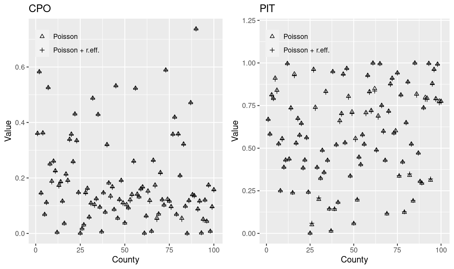
Figure 2.2: Values of CPOs and PITs computed for the models fit to the North Carolina SIDS data.

2.5 Control options

INLA has a number of arguments in the inla() function that allow us to control several options about how the estimation process is carried and the output is reported. Table 2.8 shows a summary of the different control options available in INLA. All these arguments have a manual page that can be accessed in the usual way (e.g., ?control.compute) with detailed information about the different options. In addition, the list of options for each control argument and their default values can be obtained with functions inla.set.CONTROL.default(), where CONTROL refers to the control argument. For example, for argument control.compute the list of options and default values can be obtained with inla.set.control.compute.default().

Table 2.8: Summary of control options available in INLA.

Argument	Description
control.compute	Options on what is actually computed during model fitting.
control.expert	Options on several internal issues.
control.family	Options on the likelihood of the model.
control.fixed	Options on the fixed effects of the model.
control.hazard	Options on how the hazard function is computed in survival models.
control.inla	Options on how the INLA method is used in model fitting.
control.lincomb	Options on how to compute linear combinations.
control.mode	Options on the initial values of the hyperparameters for model fitting.
control.predictor	Options on how the linear predictor is computed.
control.results	Options on the marginals to be computed.
control.update	Options on how the posterior is updated.

The different values that all these arguments can take will not be discussed here, but only wherever they are used in the book. The index at the end of the book can help to find where the different control options are used. As stated above, the documentation in the INLA package can provide full details about the different options.

It is worth mentioning that control.inla options allow the user to set the approximation used by the INLA method for model fitting described in Section 2.2. For this reason, these are covered next.

2.5.1 Model fitting strategies

Control options in control.inla can be used to set how the model is fit using the different methods described in Section 2.2. Some of the options provided by control.inla are summarized in Table 2.9.

Table 2.9: Some options in control.inla.

Option	Default	Description
strategy	'simplified.laplace'	Strategy used for the approximations (‘gaussian’, ‘simplified.laplace’, ‘laplace’ or ‘adaptive’).
int.strategy	'auto'	Integration strategy (‘auto’, ‘ccd’, ‘grid’, ‘eb’ (empirical Bayes), ‘user’ or ‘user.std’).
adaptive.max	10	Maximum length of latent effect to use the user defined strategy.
int.design	NULL	Matrix (by row) of hyperparameters values and associated weights.

Regarding the strategy used for the approximations, the options cover all the methods described before in Section 2.2. The ‘adaptive’ strategy refers to a method in which the chosen strategy is used for all fixed effects and all latent effects with a length equal or less to option adaptive.max, while all the other effects are estimated using the Gaussian approximation.

The integration strategy also covers the methods described in Section 2.2 and, in particular, Section 2.2.2. Note strategies user and user.std for user defined integration points and weights, which are provided with option int.design.

To illustrate the different approaches, the Poisson model with random effects will be fit using three different strategies as well as three different integration strategies:

m.strategy <- lapply(c("gaussian", "simplified.laplace", "laplace"), 
  function(st) {
    return(lapply(c("ccd", "grid", "eb"), function(int.st) {
      inla(SID74 ~ NWPROP74 + f(CNTY.ID, model = "iid"),
        data = nc.sids, family = "poisson", E = EXP74,
        control.inla = list(strategy = st, int.strategy = int.st),
        control.compute = list(cpo = TRUE, dic = TRUE, waic = TRUE))
    }))
})

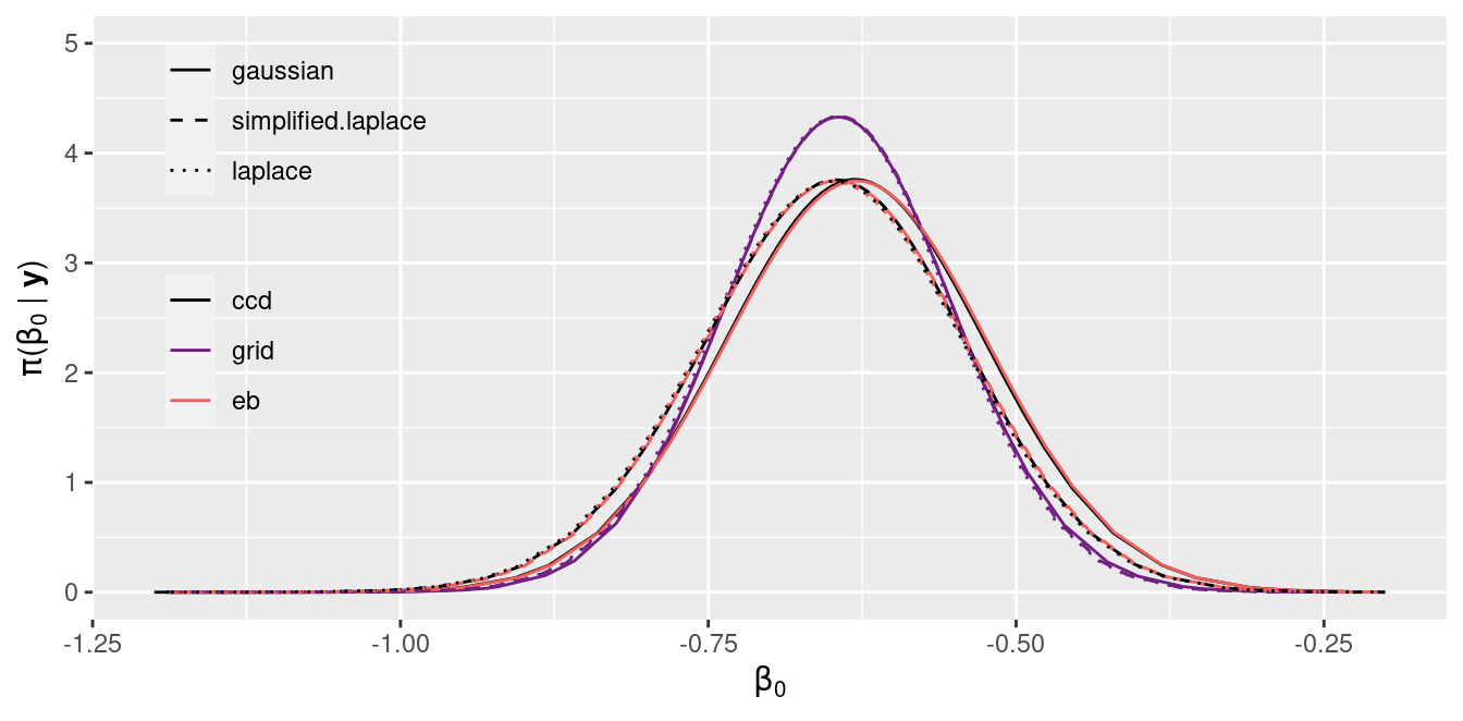
Figure 2.3: Posterior marginal of the intercept \(\beta_0\) estimated with INLA.

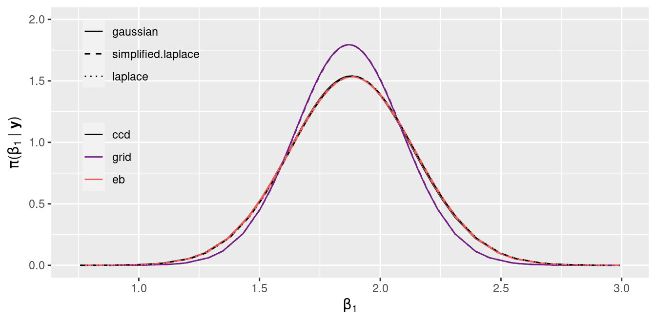
Figure 2.4: Posterior marginal of the intercept \(\beta_1\) estimated with INLA.

Figure 2.3 and Figure 2.4 show the estimates of the posterior marginal of the intercept \(\beta_0\) and the coefficient \(\beta_1\), respectively. In general, all combinations of strategy and integration strategy produce very similar results.

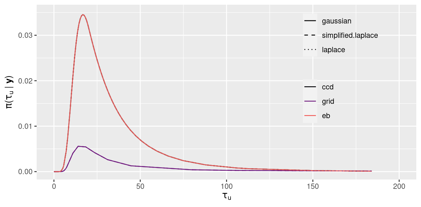
Figure 2.5: Posterior marginal of the precision of the random effects \(\tau_u\).

Figure 2.5 shows the posterior marginal of the precision of the random effects. As can be seen, the main differences are with respect to the integration strategy. The grid strategy produces results that are different to the CCD and empirical Bayes strategies. In this case, the main differences are probably due to the long tails of the grid strategy. The estimates of the posterior modes are very close for all the methods considered.

As a final comment, function inla.hyperpar() can take an inla object and improve the estimates of the posterior marginals of the hyperparameters of the model.

2.6 Working with posterior marginals

As INLA focuses on the posterior marginal distributions of the latent effects and the hyperparameters it is important to be able to exploit these for inference. INLA provides a number of functions to make computations on the posterior marginals. These are summarized in Table 2.10.

All these functions are properly documented in the INLA package manual pages. Note that a posterior marginal is a density function, and four functions to compute its density, cumulative probability, quantiles and draw random samples using the typical notation in R.

Table 2.10: Summary of functions to manipulate marginal distribution in the INLA package.

Function	Description
inla.dmarginal	Compute density function.
inla.pmarginal	Compute cumulative probability function.
inla.qmarginal	Compute a quantile.
inla.rmarginal	Draw a random sample.
inla.hpdmarginal	Compute highest posterior density (HPD) credible interval.
inla.smarginal	Spline smoothing of the posterior marginal.
inla.emarginal	Compute expected value of a function.
inla.mmarginal	Compute the posterior mode.
inla.tmarginal	Transform marginal using a function.
inla.zmarginal	Compute summary statistics.

Given a marginal \(\pi(x)\), function inla.emarginal() computes the expected value of a function \(f(x)\), i.e., \(\int f(x) \pi(x) dx\). This is useful to compute summary statistics and other quantities of interest. Typical summary statistics can be directly obtained with function inla.zmarginal(), that computes the posterior mean, standard deviation and some quantiles.

When the posterior marginal of a transformation of a latent effect or hyperparameter is required, function inla.tmarginal() can be used to transform the original posterior marginal. A typical case is to obtain the posterior marginal of the standard deviation using the posterior marginal of the precision.

As an example, we will revisit the analysis of the cement data to show how to use some of these functions. We will focus on the coefficient of covariate x1 and the precision of the Gaussian likelihood, which is a hyperparameter in the model.

First of all, the marginals of the fixed effects are stored in m1$marginals.fixed and the ones of the hyperparameters in m1$marginals.hyperpar. Both are named list identified by the corresponding name of the effect or hyperparameter. For example, the posterior marginal of the coefficient of x1 and the precision have been plotted in Figure 2.6 using

library("ggplot2")
library("gridExtra")

# Posterior of coefficient of x1
plot1 <- ggplot(as.data.frame(m1$marginals.fixed$x1)) + 
  geom_line(aes(x = x, y = y)) +
  ylab (expression(paste(pi, "(", "x", " | ", bold(y), ")")))

# Posterior of precision
plot2 <- ggplot(as.data.frame(m1$marginals.hyperpar[[1]])) + 
  geom_line(aes(x = x, y = y)) +
  ylab (expression(paste(pi, "(", tau, " | ", bold(y), ")")))

grid.arrange(plot1, plot2, nrow = 2)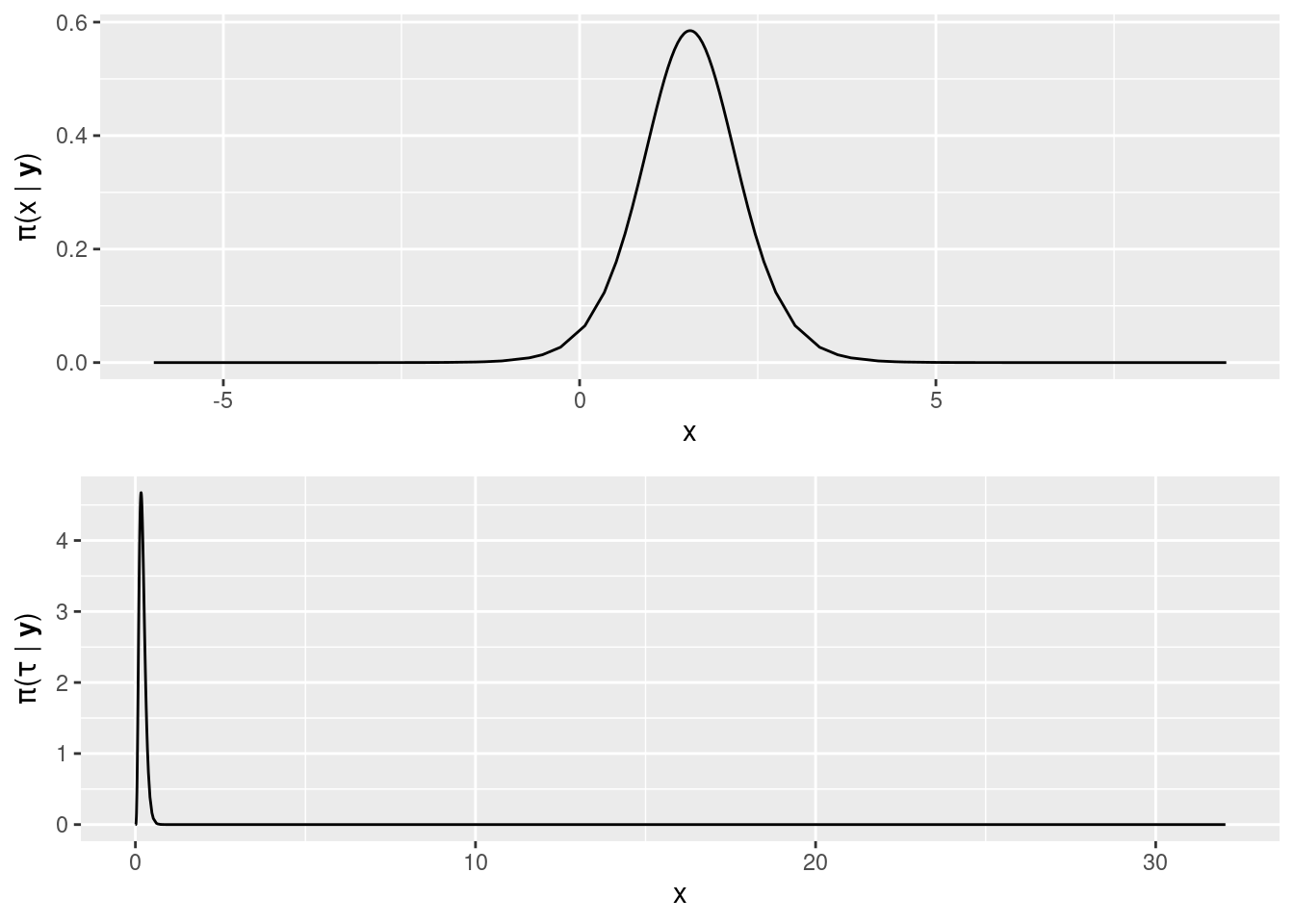

Figure 2.6: Posterior marginals of the coefficient of covariate x1 (top) and the precision of the Gaussian likelihood (bottom).

In order to know whether covariate x1 has a (positive) association with the response, the probability of its coefficient being higher than one can be computed:

1 - inla.pmarginal(0, m1$marginals.fixed$x1)

## [1] 0.9794

For the precision, an 95% highest posterior density (HPD) credible interval could be computed:

inla.hpdmarginal(0.95, m1$marginals.hyperpar[[1]])

##                low   high
## level:0.95 0.04999 0.3936

The posterior marginal of the standard deviation of the Gaussian likelihood \(\sigma_u\) can be computed by noting that the standard deviation is \(\tau_u^{-1/2}\), where \(\tau_u\) is the precision. Hence, function inla.tmarginal() can be used to transform the posterior marginal of the precision as follows:

marg.stdev <- inla.tmarginal(function(tau) tau^(-1/2),
  m1$marginals.hyperpar[[1]])

This marginal is plotted in Figure 2.7.

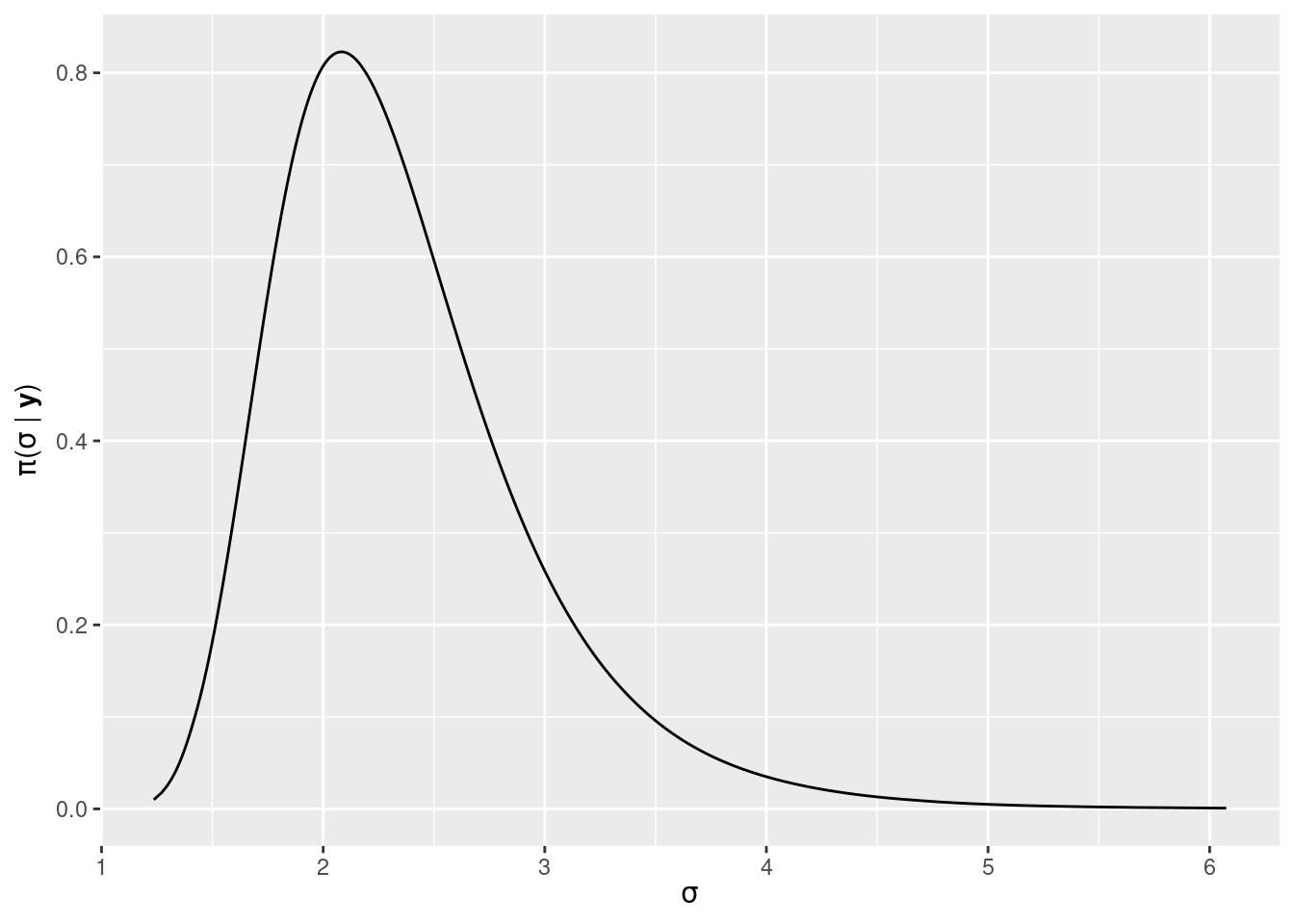
Figure 2.7: Posterior marginal of the standard deviation of the Gaussian likelihood in the linear model fit to the cement dataset.

Summary statistics from the posterior marginal of the standard deviation can be obtained with inla.zmarginal():

inla.zmarginal(marg.stdev)

## Mean            2.36854 
## Stdev           0.590885 
## Quantile  0.025 1.52821 
## Quantile  0.25  1.95203 
## Quantile  0.5   2.26194 
## Quantile  0.75  2.66324 
## Quantile  0.975 3.82571

Note that the posterior mean is \(\int \sigma \pi(\sigma \mid \mathbf{y}) d\sigma\), which could have also been computed with function inla.emarginal() as

inla.emarginal(function(sigma) sigma, marg.stdev)

## [1] 2.369

The posterior mode of the standard deviation is computed with function inla.mmarginal():

inla.mmarginal(marg.stdev)

## [1] 2.083

2.7 Sampling from the posterior

INLA can draw samples from the approximate posterior distribution of the latent effects and the hyperparameters. Function inla.posterior.sample() draws samples from the (approximate) joint posterior distribution of the latent effects and the hyperparameters. In order to use this option, the model needs to be fit with options config equal to TRUE in control.compute. This will make INLA keep the internal representation of the latent GMRF in the object returned by inla(). Furthermore, function inla.posterior.sample.eval() can be used to evaluate a function on the samples drawn.

Table 2.11 shows the different arguments that inla.posterior.sample()` can take.

Table 2.11: Arguments that can be passed to function inla.posterior.sample().

Argument	Default	Description
n	1L	Number of samples to draw.
result		An inla object.
selection		A named list with the components of the model to return.
intern	FALSE	Whether samples are in the internal scale of the hyperparameters.
use.improved.mean	TRUE	Whether to use the posterior marginal means when sampling.
add.names	TRUE	Add names of elements in each sample.
seed	0L	Seed for random number generator.
num.threads	NULL	Number of threads to be used.
verbose	FALSE	Verbose mode.

Sampling from the posterior may be useful when inference requires computing a function on the latent effects and the hyperparameters that INLA cannot handle. Non-linear functions or functions that depend on several hyperparameters that require multivariate inference for several parameters are a typical example (sse, for example, Gómez-Rubio, Bivand, and Rue 2017).

For example, we might be interested in the posterior distribution of the product of the coefficients of variables x1 and x2 in the analysis of the cement dataset. First of all, the model needs to be fit again with config equal to TRUE:

# Fit model with config = TRUE
m1 <- inla(y ~ x1 + x2 + x3 + x4, data = cement,
  control.compute = list(config = TRUE))

Next, the random sample is obtained. We will draw 100 samples from the posterior:

m1.samp <- inla.posterior.sample(100, m1, selection = list(x1 = 1, x2 = 1))

Note that here we have used the selection argument to keep just the sampled values of the coefficients of x1 and x2. Note that the expression x1 = 1 means that we want to keep the first element in effect x1. Note that in this case there is only a single value associated with x1 (i.e., the coefficient) but this can be extended to other latent random effects with possibly more values.

The object returned by inla.posterior.sample() is a list of length 100, where each element contains the samples of the different effects in the model in a name list. For example, the names for the first element of m1.samp are

names(m1.samp[[1]])

## [1] "hyperpar" "latent"   "logdens"

which correspond to the first sample of the simulated values of the hyperparameters, latent effects and the log-density of the posterior at those values. We can inspect the simulated values:

m1.samp[[1]]

## $hyperpar
## Precision for the Gaussian observations 
##                                  0.1439 
## 
## $latent
##      sample:1
## x1:1 1.300573
## x2:1 0.004523
## 
## $logdens
## $logdens$hyperpar
## [1] 1.498
## 
## $logdens$latent
## [1] 63.71
## 
## $logdens$joint
## [1] 65.21

Note that because we have used option select above there are no samples from the coefficients of covariates x3 and x4. This can be used to speed up simulations and reduce memory requirements.

Finally, function inla.posterior.sample.eval() is used to compute the product of the two coefficients:

x1x2.samp <- inla.posterior.sample.eval(function(...) {x1 * x2},
   m1.samp)

Note that the first argument is the function to be computed (using the names of the effects) and the second one the output from inla.posterior.sample. x1x2.samp is a matrix with 1 row and 100 columns so that summary statistics can be computed from the posterior as usual:

summary(as.vector(x1x2.samp))

##    Min. 1st Qu.  Median    Mean 3rd Qu.    Max. 
##  -0.445   0.013   0.809   1.502   2.026  18.102

When the interest is on the hyperparameters alone, function inla.hyperpar.sample() can be used to draw samples from the approximate joint posterior distribution of the hyperparameters. Table 2.12 shows the arguments that can be passed to this function.

Table 2.12: List of arguments that can be passed to function inla.hyperpar.sample().

Argument	Default	Description
n		Number of samples to be drawn.
result		An inla object.
intern	FALSE	Whether samples are in the internal scale of the hyperparameters.
improve.marginals	FALSE	Improve samples by using better estimates of the marginals in results.

In this case the model has only one hyperparameter (i.e., the precision of the Gaussian likelihood) and its posterior marginal could be used for inference. However, we will illustrate the use of inla.hyperpar.sample() by using it to obtain a random sample and compare its distribution of values to the posterior marginal. They should be very close.

# Sample hyperpars from joint posterior
set.seed(123)
prec.samp <- inla.hyperpar.sample(1000, m1)

Note that the returned object (prec.samp) is a matrix with as many columns as hyperparameters and a number of rows equal to the number of simulated samples. Figure 2.8 shows a histogram of the sampled values and the posterior marginal has been added for comparison purposes. Both distributions are very close. However, note that in order to validate the approximation provided by INLA it would be required to compare to other exact approaches such as MCMC. This is particularly important when the posterior marginal is very skewed. Furthermore, the samples drawn by inla.posterior.sample() rely on the approximation provided by INLA, and they should be considered as sampled from an approximation to the posterior. At the time of this writing members of the INLA team are working on providing a skewness correction for the inla.posterior.sample() function.

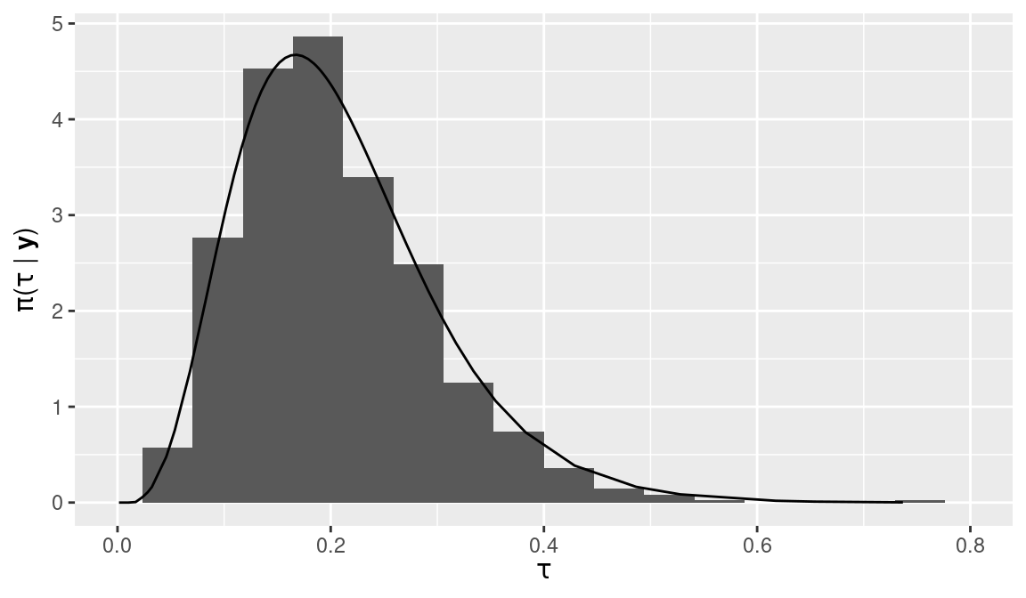
Figure 2.8: Sample from the posterior of the precision hyperparameter \(\tau\) using inla.hyperpar.sample() (histogram) and posterior marginal (solid line).

References

Bivand, Roger, Jakub Nowosad, and Robin Lovelace. 2019. SpData: Datasets for Spatial Analysis. https://CRAN.R-project.org/package=spData.

Bivand, Roger S., Edzer Pebesma, and Virgilio Gómez-Rubio. 2013. Applied Spatial Data Analysis with R. 2nd ed. New York: Springer.

Box, G. E. P., and N. R. Draper. 1987. Empirical Model Building and Response Surfaces. New York, NY: John Wiley & Sons.

Brooks, Steve, Andrew Gelman, Galin L. Jones, and Xiao-Li Meng. 2011. Handbook of Markov Chain Monte Carlo. Boca Raton, FL: Chapman & Hall/CRC Press.

Chib, S. 1995. “Marginal Likelihood from the Gibbs Output.” Journal of the American Statistical Association 90 (432): 1313–21.

Chib, S, and I Jeliazkov. 2001. “Marginal Likelihoods from the Metropolis-Hastings Output.” Journal of the American Statistical Association 96: 270–81.

Cressie, N., and N. H. Chan. 1989. “Spatial Modelling of Regional Variables.” Journal of the American Statistical Association 84: 393–401.

Cressie, N., and T. R. C. Read. 1985. “Do Sudden Infant Deaths Come in Clusters?” Statistics and Decisions, Supplement Issue 2: 333–49.

Gelman, A., X.-L. Meng, and H. Stern. 1996. “Posterior Predictive Assessment of Model Fitness via Realized Discrepancies.” Statistica Sinica 6: 733–807.

Gelman, Andrew, John B. Carlin, Hal S. Stern, David B. Dunson, Aki Vehtari, and Donald B. Rubin. 2013. Bayesian Data Analysis. 3rd ed. Boca Raton, FL: Chapman & Hall/CRC Press.

Gelman, Andrew, Jessica Hwang, and Aki Vehtari. 2014. “Understanding Predictive Information Criteria for Bayesian Models.” Statistics and Computing 24 (6): 997–1016. https://doi.org/10.1007/s11222-013-9416-2.

Gilks, W. R., W. R. Gilks, S. Richardson, and D. J. Spiegelhalter. 1996. Markov Chain Monte Carlo in Practice. Boca Raton, Florida: Chapman & Hall.

Gómez-Rubio, Virgilio, Roger S. Bivand, and Håvard Rue. 2017. “Estimating Spatial Econometrics Models with Integrated Nested Laplace Approximation.” arXiv E-Prints, March, arXiv:1703.01273. http://arxiv.org/abs/1703.01273.

Gómez-Rubio, Virgilio, and HRue. 2018. “Markov Chain Monte Carlo with the Integrated Nested Laplace Approximation.” Statistics and Computing 28 (5): 1033–51.

Gómez-Rubio, Virgilio, and Francisco Palmí-Perales. 2019. “Multivariate Posterior Inference for Spatial Models with the Integrated Nested Laplace Approximation.” Journal of the Royal Statistical Society: Series C (Applied Statistics) 68 (1): 199–215. https://doi.org/10.1111/rssc.12292.

Held, L., B. Schrödle, and H. Rue. 2010. “Posterior and Cross-Validatory Predictive Checks: A Comparison of MCMC and INLA.” In Statistical Modelling and Regression Structures – Festschrift in Honour of Ludwig Fahrmeir, edited by T. Kneib and G. Tutz, 91–110. Berlin: Springer Verlag.

Hubin, Aliaksandr, and Geir Storvik. 2016. “Estimating the marginal likelihood with integrated nested Laplace approximation (INLA).” arXiv E-Prints, November, arXiv:1611.01450. http://arxiv.org/abs/1611.01450.

MacKay, D. J. C. 2003. Information Theory, Inference, and Learning Algorithms. Cambridge University Press.

Marshall, E. C., and D. J. Spiegelhalter. 2003. “Approximate Cross-Validatory Predictive Checks in Disease Mapping Models.” Statistics in Medicine 22 (10): 1649–60.

Martins, T. G., D. Simpson, F. Lindgren, and H. Rue. 2013. “Bayesian computing with INLA: New features.” Computational Statistics & Data Analysis 67: 68–83.

Pettit, L. I. 1990. “The Conditional Predictive Ordinate for the Normal Distribution.” Journal of the Royal Statistical Society. Series B (Methodological) 52 (1): pp. 175–84.

Rue, Håvard. 2009. “INLA: An Introduction.” INLA users workshop May 2009. https://folk.ntnu.no/ingelins/INLAmai09/Pres/talkHavard.pdf.

Rue, Havard, Sara Martino, and Nicolas Chopin. 2009. “Approximate Bayesian Inference for Latent Gaussian Models by Using Integrated Nested Laplace Approximations.” Journal of the Royal Statistical Society, Series B 71 (2): 319–92.

Rue, Håvard, Andrea Riebler, Sigrunn H. Sørbye, Janine B. Illian, Daniel P. Simpson, and Finn K. Lindgren. 2017. “Bayesian Computing with INLA: A Review.” Annual Review of Statistics and Its Application 4 (1): 395–421. https://doi.org/10.1146/annurev-statistics-060116-054045.

Rue, H., and L. Held. 2005. Gaussian Markov Random Fields: Theory and Applications. Chapman; Hall/CRC Press.

Spiegelhalter, D. J., N. G. Best, B. P. Carlin, and A. Van der Linde. 2002. “Bayesian Measures of Model Complexity and Fit (with Discussion).” Journal of the Royal Statistical Society, Series B 64 (4): 583–616.

Watanabe, S. 2013. “A Widely Applicable Bayesian Information Criterion.” Journal of Machine Learning Research 14: 867–97.