Chapter 7 Spatial Models
7.1 Introduction
Many models assume that observations are obtained independently of each other. However, this is seldom the case. In Chapter 4 we have already seen how to account for correlated observations within groups. Distance between observations can also be a source of correlation. For example, in a city housing value usually changes smoothly between too contiguous neighborhoods. Pollution also shows a spatial smooth pattern and measurements close in space will likely be very similar. Also, the location of trees in a forest may follow a spatial pattern, depending on ground conditions, soil nutrients, etc.
All these examples have in common the spatial nature of the data. Observations that are close in space are likely to show similar values and a high degree of spatial autocorrelation. Spatial models will take into account this spatial autocorrelation in order to separate the general trend (usually depending on some covariates) from the purely spatial random variation.
Spatial statistics is traditionally divided into three main areas depending on
the type of problem and data: lattice data, geostatistics and point patterns
(Cressie 2015). Sometimes, spatial data is also measured over time and
spatio-temporal models can be proposed (Cressie and Wikle 2011). In the next
sections models for the different types of spatial data will be considered.
In Section 8.6 models for spatio-temporal data will
be described. Blangiardo and Cameletti (2015) and Krainski et al. (2018) provide
a thorough description of most of the models described in this section.
Bivand, Pebesma, and Gómez-Rubio (2013) and Lovelace, Nowosad, and Muenchow (2019) provide general description on
handling spatial data in R and are recommended reads.
Spatial models for spatial data are introduced in Section 7.2. Geostatistical models for continuous spatial processes are presented in Section 7.3. Next, the analysis of point patterns is described in 7.4.
7.2 Areal data
Areal data, also known as lattice data, usually refers to data that are observed within given boundaries. For example, administrative boundaries are often used and the variables of study aggregated over these regions. Administrative boundaries will produce a lattice which will often have an irregular structure. Lattices with regular structures are difficult to find, but they may appear when spatial data come from an experiment (as described below).
In either case, spatial adjacency is often represented by a (sparse) adjacency matrix, with non-zero entries at the intersection of rows and columns of neighboring areas. This matrix will play an important role when building spatial models as spatial correlation structures will be built upon it. In particular, spatially correlated random effects will be modeled using a multivariate Gaussian distribution with a precision matrix that depends on an adjacency matrix.
7.2.1 Regular lattice
A regular lattice occurs when areas are structured as a matrix in rows and columns. It is often the case that spatial data is in a regular lattice as a result of an experimental design or data collection structure. For example, a regular lattice is a convenient way of modeling a count process, so that the study region is divided into small squares and the number of events in each cell is recorded. Because of the spatially inhomogeneous distribution of the events, cells which are neighbors will tend to have a similar number of events and this is how spatial autocorrelation appears in these data.
The bei dataset in the spatstat package (Baddeley, Rubak, and Turner 2015) records the
locations of 3605 trees in a tropical rain forest
(Condit 1998; Condit, Hubbell, and Foster 1996; Hubbell and Foster 1983; Møller and Waagepetersen 2007).
This is stored as a ppp object, that essentially contains the boundary of the
study region, a \(1000 \times 500\) meters region in this case, and the
coordinates of the points. Furthermore, the bei.extra dataset includes the
elevation and slope in the study region. These are available as im objects,
which are raster images that cover the study area. Each raster is made of
\(201\times 101\) pixels that represent the study area.
A regular lattice can be created from the original data by considering
a matrix of \(5 \times 10\) squares in which the number of trees inside
is computed. The following code makes extensive use of function in the
sp and spatstat packages.
First of all, dataset bei is loaded and converted into a SpatialPoints
object to represent the point pattern using classes in the sp package:
library("spatstat")
library("sp")
library("maptools")

data(bei)

# Create SpatialPoints object
bei.pts <- as(bei, "SpatialPoints")
Next, a grid over the rectangular study region is created to count the number of trees inside each of the cells in the grid:
#Create grid
bei.poly <- as(as.im(bei$window, dimyx=c(5, 10)), "SpatialGridDataFrame")
bei.poly <- as(bei.poly, "SpatialPolygons")
Function over() is used now to overlay the point pattern and the cells in
the grid, so that the number of points in each cell of the grid is obtained.
#Number of observations per cell
idx <- over(bei.pts, bei.poly)
tab.idx <- table(idx)
#Add number of trees
d <- data.frame(Ntrees = rep(0, length(bei.poly)))
row.names(d) <- paste0("g", 1:length(bei.poly))
d$Ntrees[as.integer(names(tab.idx))] <- tab.idx
Finally, a SpatialPolygonsDataFrame is created by putting together
the polygon representation of the cells in the grid and the number of
trees in each cell:
#SpatialPolygonsDataFrame
bei.trees <- SpatialPolygonsDataFrame(bei.poly, d)
At this point, it is important to highlight how spatial data is internally
stored in a SpatialGridDataFrame and the latent effects described in Table
7.1. For some models, INLA considers data sorted by
column, i.e., a vector with the first column of the grid from top to bottom,
followed by the second column and so on. In order to have this mapping we need
to reorder the data as follows:
#Mapping
idx.mapping <- as.vector(t(matrix(1:50, nrow = 10, ncol = 5)))
bei.trees2 <- bei.trees[idx.mapping, ]
Figure 7.1 shows the order in which observations are internally
stored in a SpatialGridDataFrame and how they are considered by the models
in Table 7.1.
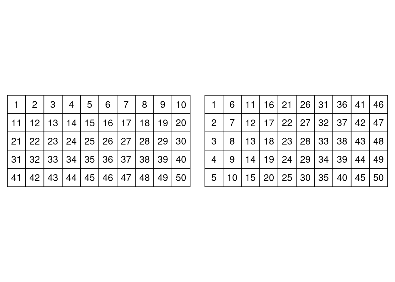
Figure 7.1: Mapping of cells in a SGDF (left) and mapping required by INLA (right).
Figure 7.2 represents the cells into which we have divided the study region, that have been colored according to the number of trees inside. Furthermore, the actual location of the points has been plotted as an extra spatial layer to assess that the counts are correct.
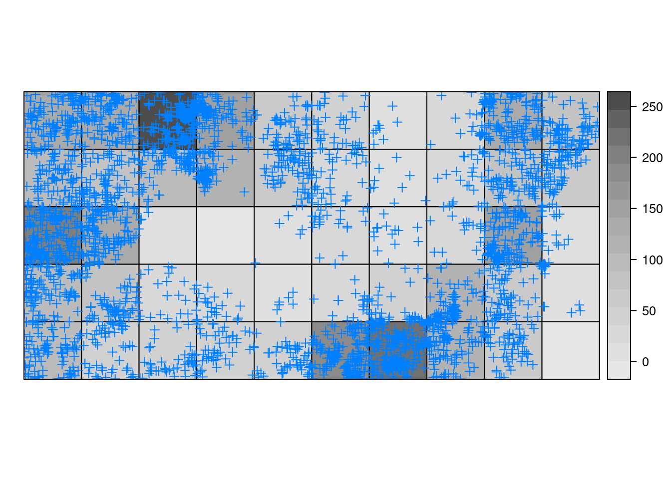
Figure 7.2: Spatial distribution of trees in a rain forest.
In addition to the counts, we will obtain summary statistics of the covariates to be used in our model fitting.
#Summary statistics of covariates
covs <- lapply(names(bei.extra), function(X) {
  layer <- bei.extra[[X]]
    res <- lapply(1:length(bei.trees2), function(Y) {
      summary(layer[as.owin(bei.trees2[Y, ])])})
    res <- as.data.frame(do.call(rbind, res))

    names(res) <- paste0(X, ".", c("min", "1Q", "2Q", "mean", "3Q", "max"))
    return(res)
    })

covs <- do.call(cbind, covs)

#Add to SPDF
bei.trees2@data <- cbind(bei.trees2@data, covs)
Figure 7.3 shows the average values of the elevation and gradient in the cells. When areal data are considered, aggregating individual data over areas is useful to build regression models. However, this aggregation process may blur the underlying point process.
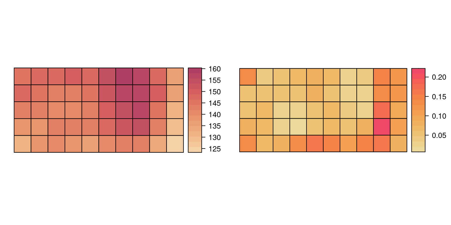
Figure 7.3: Average values of elevation (left) and gradient (right).
Spatial models for lattice data are often defined as random effects with a
variance-covariance structure that depends on the neighborhood structure of the
areas. In general, two areas will be neighbors if they share some boundaries.
This could be just a single point (i.e., queen adjacency) or at least
a segment (rook adjacency). For the current dataset, this is illustrated
in Figure 7.4. The neighborhood structure has been obtained
with function poly2nb from package spdep (Bivand and Wong 2018), which will return an
nb object.
library("spdep")
library("spatialreg")
bei.adj.q <- poly2nb(bei.trees2)
bei.adj.r <- poly2nb(bei.trees2, queen = FALSE)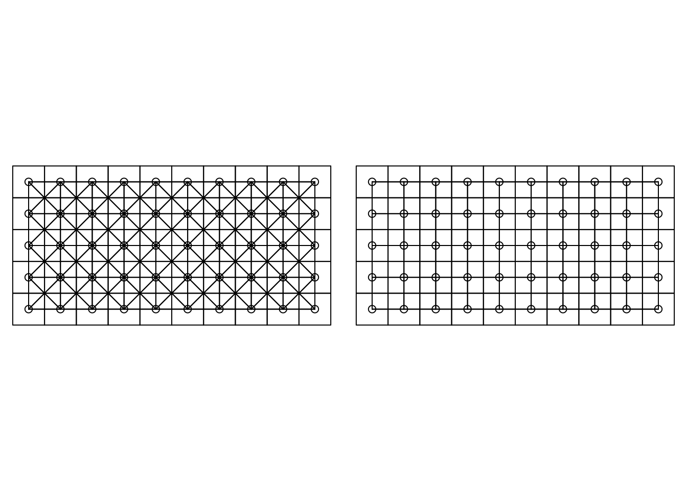
Figure 7.4: Queen (left) versus rook (right) adjacency.
For \(n\) regions, adjacency can be represented as a \(n \times n\) matrix with
non-zero entries if the regions in that row and column are neighbors. This
is often represented as a binary indicator, but other types of weights can
be used. Function nb2listw can be used to transform an nb object into
a matrix of spatial weights using different specifications. A matrix
of spatial weights will be denoted by \(W\).
The following code will create two adjacency matrices with binary weights
(style = "B") and row-standardized (style = "W"), so that the values in
each row sum up to one:
W.bin <- nb2listw(bei.adj.q, style = "B")
W.rs <- nb2listw(bei.adj.q, style = "W")
W.bin
## Characteristics of weights list object:
## Neighbour list object:
## Number of regions: 50
## Number of nonzero links: 314
## Percentage nonzero weights: 12.56
## Average number of links: 6.28
##
## Weights style: B
## Weights constants summary:
## n nn S0 S1 S2
## B 50 2500 314 628 8488W.rs## Characteristics of weights list object:
## Neighbour list object:
## Number of regions: 50
## Number of nonzero links: 314
## Percentage nonzero weights: 12.56
## Average number of links: 6.28
##
## Weights style: W
## Weights constants summary:
## n nn S0 S1 S2
## W 50 2500 50 16.82 203.4Spatial latent effects are multivariate Gaussian distribution with zero mean and precision matrix \(\tau \Sigma\), where \(\tau\) is an hyperparameter (i.e., the precision) and \(\Sigma\) a matrix that depends on the spatial adjacency matrix \(W\). Depending on the complexity of the spatial effect, matrix \(\Sigma\) may also depend on further hyperparameters (Banerjee, Carlin, and Gelfand 2014).
A summary of the main spatial latent effects available in INLA for regular
lattice data is available in Table 7.1.
| Model | Precision |
|---|---|
rw2d |
Random walk of order 2. |
matern2d |
Gaussian field with Matérn correlation. |
First of all, non-spatial models using the covariates and i.i.d. Gaussian random effects will be fit. This will serve as a baseline in order to assess whether spatial dependence is really needed in the model.
library("INLA")

#Log-Poisson regression
m0 <- inla(Ntrees ~ elev.mean + grad.mean, family = "poisson",
  data = as.data.frame(bei.trees2) )

#Log-Poisson regression with random effects
bei.trees2$ID <- 1:length(bei.trees2)
m0.re <- inla(Ntrees ~ elev.mean + grad.mean + f(ID), family = "poisson",
  data = as.data.frame(bei.trees2) )
As noted above, INLA assumes that the lattice is stored by columns, i.e., a
vector with the first column, then followed by the second column and so on.
Hence, a proper mapping between the spatial object with the data and the
data.frame used in the call to inla is required.
In this case, data have already been reordered to the right mapping and the model can be fitted:
#RW2d
m0.rw2d <- inla(Ntrees ~ elev.mean + grad.mean +
    f(ID, model = "rw2d", nrow = 5, ncol = 10),
  family = "poisson", data = as.data.frame(bei.trees2),
  control.predictor = list(compute = TRUE),
  control.compute = list(dic = TRUE) )

summary(m0.rw2d)
##
## Call:
## c("inla(formula = Ntrees ~ elev.mean + grad.mean + f(ID, model =
## \"rw2d\", ", " nrow = 5, ncol = 10), family = \"poisson\", data =
## as.data.frame(bei.trees2), ", " control.compute = list(dic =
## TRUE), control.predictor = list(compute = TRUE))" )
## Time used:
## Pre = 0.225, Running = 0.125, Post = 0.0244, Total = 0.374
## Fixed effects:
## mean sd 0.025quant 0.5quant 0.975quant mode kld
## (Intercept) -10.863 7.781 -26.360 -10.821 4.391 -10.737 0
## elev.mean 0.094 0.053 -0.010 0.094 0.200 0.094 0
## grad.mean 12.652 3.566 5.619 12.648 19.704 12.638 0
##
## Random effects:
## Name Model
## ID Random walk 2D
##
## Model hyperparameters:
## mean sd 0.025quant 0.5quant 0.975quant mode
## Precision for ID 0.242 0.066 0.135 0.235 0.393 0.22
##
## Expected number of effective parameters(stdev): 45.08(0.862)
## Number of equivalent replicates : 1.11
##
## Deviance Information Criterion (DIC) ...............: 385.18
## Deviance Information Criterion (DIC, saturated) ....: 109.38
## Effective number of parameters .....................: 45.27
##
## Marginal log-Likelihood: -319.68
## Posterior marginals for the linear predictor and
## the fitted values are computed#Matern2D
m0.m2d <- inla(Ntrees ~ elev.mean + grad.mean +
f(ID, model = "matern2d", nrow = 5, ncol = 10),
family = "poisson", data = as.data.frame(bei.trees2),
control.predictor = list(compute = TRUE) )
summary(m0.m2d)##
## Call:
## c("inla(formula = Ntrees ~ elev.mean + grad.mean + f(ID, model =
## \"matern2d\", ", " nrow = 5, ncol = 10), family = \"poisson\",
## data = as.data.frame(bei.trees2), ", " control.predictor =
## list(compute = TRUE))")
## Time used:
## Pre = 0.228, Running = 0.225, Post = 0.0251, Total = 0.477
## Fixed effects:
## mean sd 0.025quant 0.5quant 0.975quant mode kld
## (Intercept) -8.463 3.977 -16.449 -8.415 -0.756 -8.320 0
## elev.mean 0.079 0.028 0.026 0.079 0.134 0.078 0
## grad.mean 14.119 3.347 7.595 14.092 20.793 14.040 0
##
## Random effects:
## Name Model
## ID Matern2D model
##
## Model hyperparameters:
## mean sd 0.025quant 0.5quant 0.975quant mode
## Precision for ID 0.354 0.24 0.037 0.306 0.895 0.114
## Range for ID 8.063 5.50 3.294 6.377 22.747 4.223
##
## Expected number of effective parameters(stdev): 45.94(0.719)
## Number of equivalent replicates : 1.09
##
## Marginal log-Likelihood: -274.11
## Posterior marginals for the linear predictor and
## the fitted values are computedOnce the models have been fit, the posterior means
of the fitted values are added to the SpatialPolygonsDataFame
for plotting:
bei.trees2$RW2D <- m0.rw2d$summary.fitted.values[, "mean"]

bei.trees2$MATERN2D <- m0.m2d$summary.fitted.values[, "mean"]
As a summary of the fit models, Figure 7.5 shows
the posterior means of the spatial random effects for the rw2d and
matern2d models. The results support the hypothesis of a non-uniform
distribution of the trees in the region.
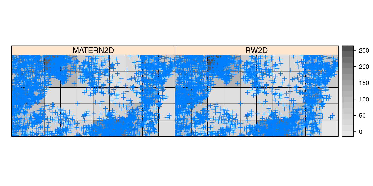
Figure 7.5: Posterior means of fitted values for regular lattices for the bei dataset.
7.2.2 Irregular lattice
Lattice data are seldom in a regular grid. For example, administrative
boundaries usually lead to an irregular lattice. The boston dataset,
available in the spData package, records housing values in Boston census
tracts (Harrison and Rubinfeld 1978) corrected for a few errors (Gilley and Pace 1996)
and including longitude and latitude of the observations (Bivand 2017).
Table 7.2 describes the variables in the dataset.
| Variable | Description |
|---|---|
TOWN |
Town name |
CMEDV |
Corrected median of owner-occupied housing (in USD 1,000) |
CRIM |
Crime per capita |
ZN |
Proportions of residential land zoned for lots over 25,000 sq. ft per town |
INDUS |
Proportions of non-retail business acres per town |
CHAS |
Whether the tract borders Charles river (1 = yes, 0 = no) |
NOX |
Nitric oxides concentration (in parts per 10 million) |
RM |
Average number of rooms per dwelling |
AGE |
Proportions of owner-occupied units built prior to 1940 |
DIS |
Weighted distances to five Boston employment centres |
RAD |
Index of accesibility to radial highways per town |
TAX |
Full-value property-tax rate per USD 10,000 per town |
PTRATIO |
Pupil-teacher ratios per town |
B |
\(1000*(Bk - 0.63)^2\), where \(Bk\) is the proportion of blacks |
LSTAT |
Percentage values of lower status population |
This dataset is available as a shapefile in the spData package,
that can be loaded as follows:
library("rgdal")
boston.tr <- readOGR(system.file("shapes/boston_tracts.shp",
  package="spData")[1])
In order to compute the adjacency matrix, function poly2nb can be used:
boston.adj <- poly2nb(boston.tr)By default, it will create a binary adjacency matrix, so that two regions are neighbors only if they share at least one point in common boundary (i.e., it is a queen adjacency). Figure 7.6 shows Boston census tracts in the data and the adjacency matrix.
Because of the irregular nature of the adjacency structure of the census tracts, the models introduced in the previous section cannot be used. Furthermore, binary and row-standardized adjacency matrices will be computed as they will be needed by the spatial models presented below:
W.boston <- nb2mat(boston.adj, style = "B")
W.boston.rs <- nb2mat(boston.adj, style = "W")
This dataset contains a few censored observations in the response, which
correspond to tracts with a higher median housing value then $50,000. For
this reason, we will set all values equal to \(50.0\) to NA. This means that
these areas will not be used for model fitting, but the predictive distribution
will be computed by INLA so that inference on the housing value in these areas
is still possible. See Section 12.3 for more details about how
the predictive distribution is computed.
boston.tr$CMEDV2 <- boston.tr$CMEDV
boston.tr$CMEDV2 [boston.tr$CMEDV2 == 50.0] <- NA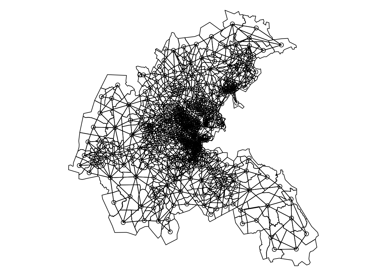
Figure 7.6: Boston tracts and adjacency matrix.
The model that we will be fitting will consider the response in the log-scale
as this will make the response less skewed. The formula with the 13 covariates
included in the model can be seen below. This is similar to the analysis
performed in Harrison and Rubinfeld (1978) but other random effects will be
considered as well to illustrate the use of the different models. In addition,
a new column with the a region ID will be added to be used when defining
random effects.
boston.form  <- log(CMEDV2) ~ CRIM + ZN + INDUS + CHAS + I(NOX^2) + I(RM^2) +
    AGE + log(DIS) + log(RAD) + TAX + PTRATIO + B + log(LSTAT)
boston.tr$ID <- 1:length(boston.tr)
First of all, a model with i.i.d. random effects will be fit to the data.
This will provide a baseline to assess whether spatial random effects
are really required when modeling these data. The estimates of the
random effects (i.e., posterior means) will be added to the
SpatialPolygonsDataFrame to be plotted later.
boston.iid <- inla(update(boston.form, . ~. + f(ID, model = "iid")),
  data = as.data.frame(boston.tr),
  control.compute = list(dic = TRUE, waic = TRUE, cpo = TRUE),
  control.predictor = list(compute = TRUE)
)
summary(boston.iid)
##
## Call:
## c("inla(formula = update(boston.form, . ~ . + f(ID, model =
## \"iid\")), ", " data = as.data.frame(boston.tr), control.compute =
## list(dic = TRUE, ", " waic = TRUE, cpo = TRUE), control.predictor
## = list(compute = TRUE))" )
## Time used:
## Pre = 0.39, Running = 1.48, Post = 0.0545, Total = 1.92
## Fixed effects:
## mean sd 0.025quant 0.5quant 0.975quant mode kld
## (Intercept) 4.376 0.151 4.080 4.376 4.672 4.376 0
## CRIM -0.011 0.001 -0.013 -0.011 -0.009 -0.011 0
## ZN 0.000 0.000 -0.001 0.000 0.001 0.000 0
## INDUS 0.001 0.002 -0.003 0.001 0.006 0.001 0
## CHAS1 0.056 0.034 -0.010 0.056 0.123 0.056 0
## I(NOX^2) -0.540 0.107 -0.751 -0.540 -0.329 -0.540 0
## I(RM^2) 0.007 0.001 0.005 0.007 0.010 0.007 0
## AGE 0.000 0.001 -0.001 0.000 0.001 0.000 0
## log(DIS) -0.143 0.032 -0.206 -0.143 -0.080 -0.143 0
## log(RAD) 0.082 0.018 0.047 0.082 0.118 0.082 0
## TAX 0.000 0.000 -0.001 0.000 0.000 0.000 0
## PTRATIO -0.031 0.005 -0.040 -0.031 -0.021 -0.031 0
## B 0.000 0.000 0.000 0.000 0.001 0.000 0
## log(LSTAT) -0.329 0.027 -0.382 -0.329 -0.277 -0.329 0
##
## Random effects:
## Name Model
## ID IID model
##
## Model hyperparameters:
## mean sd 0.025quant
## Precision for the Gaussian observations 34.42 2.23 30.19
## Precision for ID 18666.46 18355.20 1250.33
## 0.5quant 0.975quant mode
## Precision for the Gaussian observations 34.36 38.98 34.27
## Precision for ID 13249.17 67299.69 3412.82
##
## Expected number of effective parameters(stdev): 18.53(10.17)
## Number of equivalent replicates : 26.45
##
## Deviance Information Criterion (DIC) ...............: -325.37
## Deviance Information Criterion (DIC, saturated) ....: 508.04
## Effective number of parameters .....................: 18.81
##
## Watanabe-Akaike information criterion (WAIC) ...: -317.68
## Effective number of parameters .................: 25.46
##
## Marginal log-Likelihood: 42.81
## CPO and PIT are computed
##
## Posterior marginals for the linear predictor and
## the fitted values are computedNote that the model is fit on the logarithm of CMEDV2. Hence, in order to
make inference about CMEDV2 directly, the posterior marginals of the fitted
values need to be transform with function inla.tmarginal() and then the
posterior mean computed with inla.emarginal() (see Section
2.6 for details on manipulating marginals distributions). A
new function tmarg()will be created to be used by other models as well.
# Use 4 cores to process marginals in parallel
library("parallel")
options(mc.cores = 4)
# Transform marginals and compute posterior mean
#marginals: List of `marginals.fitted.values`from inla model
tmarg <- function(marginals) {
  post.means <- mclapply(marginals, function (marg) {
  # Transform post. marginals
  aux <- inla.tmarginal(exp, marg)
  # Compute posterior mean
  inla.emarginal(function(x) x, aux)
  })

  return(as.vector(unlist(post.means)))
}

# Add posterior means to the SpatialPolygonsDataFrame

boston.tr$IID <- tmarg(boston.iid$marginals.fitted.values)
Regarding spatial models for data in an irregular lattice, Table
7.3 summarizes some of the models available in INLA.
| Model | Precision |
|---|---|
besagproper |
Proper version of Besag’s spatial model |
besag |
Besag’s spatial model (improper prior) |
bym |
Convolution model, i.e., besag plus iid models |
Three models will be considered: Besag’s proper spatial model, Besag’s improper spatial model and the one by Besag, York and Mollié, that is a convolution of an intrinsic CAR model and i.i.d. Gaussian model:
#Besag's improper
boston.besag <- inla(update(boston.form, . ~. +
    f(ID, model = "besag", graph = W.boston)),
  data = as.data.frame(boston.tr),
  control.compute = list(dic = TRUE, waic = TRUE, cpo = TRUE),
  control.predictor = list(compute = TRUE)
)
boston.tr$BESAG <- tmarg(boston.besag$marginals.fitted.values)


#Besag proper
boston.besagprop <- inla(update(boston.form, . ~. +
    f(ID, model = "besagproper", graph = W.boston)),
  data = as.data.frame(boston.tr),
  control.compute = list(dic = TRUE, waic = TRUE, cpo = TRUE),
  control.predictor = list(compute = TRUE)
)
boston.tr$BESAGPROP <- tmarg(boston.besagprop$marginals.fitted.values)


#BYM
boston.bym <- inla(update(boston.form, . ~. +
    f(ID, model = "bym", graph = W.boston)),
  data = as.data.frame(boston.tr),
  control.compute = list(dic = TRUE, waic = TRUE, cpo = TRUE),
  control.predictor = list(compute = TRUE)
)
boston.tr$BYM <- tmarg(boston.bym$marginals.fitted.values)
A convenient model when the aim is to assess spatial dependence in the data is the one proposed in Leroux, Lei, and Breslow (1999). In this model, the structure of the precision matrix is a convex combination of an identity matrix \(I\) (to represent i.i.d. spatial effect) and the precision of an intrinsic CAR \(Q\) (to represent a spatial pattern):
\[ (1 - \lambda) I + \lambda Q \]
Parameter \(\lambda\) lies between 0 and 1 and it controls the amount of spatial structure in the data. Small values indicate a non-spatial pattern, while large values indicate a strong spatial pattern.
Although this model is not directly implemented in INLA it can be noted that
it is possible to fit this model using the generic1 (see Section
3.3) by taking matrix \(C\) equal to \(I - Q\), where \(Q\) is the
precision matrix of an intrinsic CAR specification
(Ugarte et al. 2014; Bivand, Gómez-Rubio, and Rue 2015).
Q <- Diagonal(x = sapply(boston.adj, length))
Q <- Q - as_dsTMatrix_listw(nb2listw(boston.adj, style = "B"))

C <- Diagonal(x = 1, n = nrow(boston.tr)) - Q
boston.ler <- inla(update(boston.form, . ~. +
f(ID, model = "generic1", Cmatrix = C)),
data = as.data.frame(boston.tr),
control.compute = list(dic = TRUE, waic = TRUE, cpo = TRUE),
control.predictor = list(compute = TRUE)
)
boston.tr$LER <- tmarg(boston.ler$marginals.fitted.values)Figure 7.7 displays the observed values of CMEDV2 and
the point estimates obtained with the different models. In the plot for
CMEDV2 a few holes can be seen, which are filled with the prediction from the
different models in the other plots. In the models with spatially correlated
random effects this prediction is based on the covariates plus the spatially
correlated random effects.
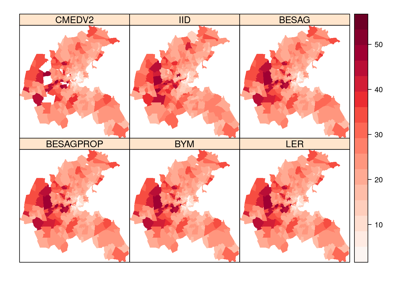
Figure 7.7: Summary of observed data and posterior means obtained with different models for the Boston housing dataset.
In general, all models provide similar posterior point estimates of the median housing value. For the areas with censored data, the predictive distributions also provide very similar estimates.
In terms of model selection criteria (see Section 2.4), Table 7.5 shows the different values for each model. All criteria point to the model by Leroux, Lei, and Breslow (1999) as the best one.
| Model | DIC | WAIC | CPO |
|---|---|---|---|
iid |
-325.4 | -317.7 | -158.2 |
| besag | -2185.7 | -2185.7 | -692.8 |
| besagproper | -2694.7 | -2694.7 | -775.2 |
| bym | -2844.9 | -2844.9 | -953.4 |
| leroux | -2795.4 | -2795.4 | -909.4 |
Table: (#tab:bostonmodsel) Summary of model selection criteria of the models fit to the Boston housing dataset .
7.3 Geostatistics
Geostatistics deals with the analysis of continuous processes in space. A typical example is the spatial distribution of temperature or pollutants in the air. In this case, the variable of interest is only observed at a finite number of points and statistical methods are required for estimation all over the study region.
A geostatistical process is often represented as a continuous stochastic process \(y(x)\) with \(x\in \mathcal{D}\), where \(\mathcal{D}\) is the study region. This stochastic process is often assumed to follow a Gaussian distribution and \(y(x)\) is then called a Gaussian Process (GP, Cressie 2015).
In principle, dependence between two observations of the GP can be modeled by using an appropriate covariance function. However, quite often the GP is assumed to fulfill two important properties. First of all, the GP is assumed to be stationary, which means that the covariance between two points is the same even if they are shifted in space. Furthermore, the GP is assumed to be isotropic, which means that the correlation between two observations only depends on the distance between them. Making these two assumptions simplifies modeling of the geostatistics process as the covariance between two points will only depend on the relative distance between them regardless of their relative positions.
A commonly used covariance function is the Matérn covariance function (Cressie 2015). The covariance of two points which are a distance \(d\) apart is:
\[ C_{\nu} (d) = \sigma^2 \frac{2^{1 - \nu}}{\Gamma(\nu)} \left(\sqrt{2\nu}\frac{d}{\rho}\right)^{\nu} K_{\nu}\left(\sqrt{2\nu}\frac{d}{\rho}\right) \]
Here, \(\Gamma(\cdot)\) is the gamma function and \(K_{\nu}(\cdot)\) is the modified Bessel function of the second kind. Parameters \(\sigma^2\), \(\rho\) and \(\nu\) are non-negative values of the covariance function.
Parameter \(\sigma^2\) is a general scale parameter. The range of the spatial process is controlled by parameter \(\rho\). Large values will imply a fast decay in the correlation with distance, which imply a small range spatial process. Small values will indicate a spatial process with a large range. Finally, parameter \(\nu\) controls smoothness of the spatial process.
7.3.1 The meuse dataset
The meuse dataset in package gstat (Pebesma 2004) contains measurements of
heavy metals concentrations in the fields next to the Meuse river, near the
village of Stein (The Netherlands). In addition, the meuse.grid dataset
records several of the covariates in the meuse dataset in a regular grid over
the study region. These can be used in order to estimate the concentration
of heavy metals at any point of the study region.
| Variable | Description |
|---|---|
x |
Easting (in meters). |
y |
Northing (in meters). |
cadmium |
Topsoil cadmium concentration (in ppm). |
copper |
Topsoil copper concentration (in ppm). |
lead |
Topsoil lead concentration (in ppm). |
zinc |
Topsoil zinc concentration (in ppm). |
elev |
Relative elevation above local river bed (in meters). |
dist |
Distance to the Meuse river (normalized to \([0, 1]\)). |
om |
Organic matter (in percentage). |
ffreq |
Flooding frequency (1 = once in two years; 2 = once in ten years; 3 = once in 50 years). |
soil |
Soil type (1 = Rd10A; 2 = Rd90C/VII; 3 = Bkd26/VII). |
lime |
Lime class (0 = absent; 1 = present). |
landuse |
Land use class. |
dist.m |
Distance to the river (in meters). |
These two datasets can be loaded by following the commands listed in their respective manual pages:
library("gstat")
data(meuse)

summary(meuse)
## x y cadmium copper
## Min. :178605 Min. :329714 Min. : 0.20 Min. : 14.0
## 1st Qu.:179371 1st Qu.:330762 1st Qu.: 0.80 1st Qu.: 23.0
## Median :179991 Median :331633 Median : 2.10 Median : 31.0
## Mean :180005 Mean :331635 Mean : 3.25 Mean : 40.3
## 3rd Qu.:180630 3rd Qu.:332463 3rd Qu.: 3.85 3rd Qu.: 49.5
## Max. :181390 Max. :333611 Max. :18.10 Max. :128.0
##
## lead zinc elev dist
## Min. : 37.0 Min. : 113 Min. : 5.18 Min. :0.0000
## 1st Qu.: 72.5 1st Qu.: 198 1st Qu.: 7.55 1st Qu.:0.0757
## Median :123.0 Median : 326 Median : 8.18 Median :0.2118
## Mean :153.4 Mean : 470 Mean : 8.16 Mean :0.2400
## 3rd Qu.:207.0 3rd Qu.: 674 3rd Qu.: 8.96 3rd Qu.:0.3641
## Max. :654.0 Max. :1839 Max. :10.52 Max. :0.8804
##
## om ffreq soil lime landuse dist.m
## Min. : 1.00 1:84 1:97 0:111 W :50 Min. : 10
## 1st Qu.: 5.30 2:48 2:46 1: 44 Ah :39 1st Qu.: 80
## Median : 6.90 3:23 3:12 Am :22 Median : 270
## Mean : 7.48 Fw :10 Mean : 290
## 3rd Qu.: 9.00 Ab : 8 3rd Qu.: 450
## Max. :17.00 (Other):25 Max. :1000
## NA's :2 NA's : 1Next, we will create a SpatialPointsDataFrame and assign the data
its coordinate reference system (obtained from the manual page):
coordinates(meuse) <- ~x+y
proj4string(meuse) <- CRS("+init=epsg:28992")
A similar operation will be performed on the grid. Note that now the
resulting object is a SpatialPixelsDataFrame, which is one of the objects in
the sp package to represent spatial grids:
#Code from gstat
data(meuse.grid)
coordinates(meuse.grid) = ~x+y
proj4string(meuse.grid) <- CRS("+init=epsg:28992")
gridded(meuse.grid) = TRUE
Note that function proj4string is used to set the correct coordinate
reference system (CRS) for the data, which essentially sets the units of the
coordinates of the points as these do not necessarily need to be longitude and
latitude. In this case, the CRS is Netherlands topographical map coordinates
and they are measured in meters.
7.3.2 Kriging
As a preliminary analysis of this dataset, kriging will be used to obtain an estimation of the concentration of zinc in the study region. In particular, universal kriging (Cressie 2015; Bivand, Pebesma, and Gómez-Rubio 2013) will be used in order to include covariates in the prediction.
First of all, the empirical variogram will be computed using function
variogram() and a spherical variogram fitted using function
fit.variogram.
# Variogram and fit variogram
vgm <- variogram(log(zinc) ~ dist, meuse)
fit.vgm <- fit.variogram(vgm, vgm("Sph"))
Next, universal kriging will provide an estimate of the concentration of zinc
at all points of the grid defined in meuse.grid. In addition to the point
estimates, the square root of the prediction variance (which can be used as a
measure of the error in the prediction) will be added as well.
# Kriging
krg <- krige(log(zinc) ~ dist, meuse, meuse.grid, model = fit.vgm)
## [using universal kriging]#Add estimates to meuse.grid
meuse.grid$zinc.krg <- krg$var1.pred
meuse.grid$zinc.krg.sd <- sqrt(krg$var1.var)Figure 7.8 shows the concentration of zinc, in the log-scale, estimated using universal kriging. The plot shows a clear spatial pattern, with higher concentrations in points closer to the Meuse river. These estimates will be compared later to other estimates obtained with spatial models fit with INLA. Note that the standard errors of the estimates have been computed and will be compared later to their analogous Bayesian estimates.
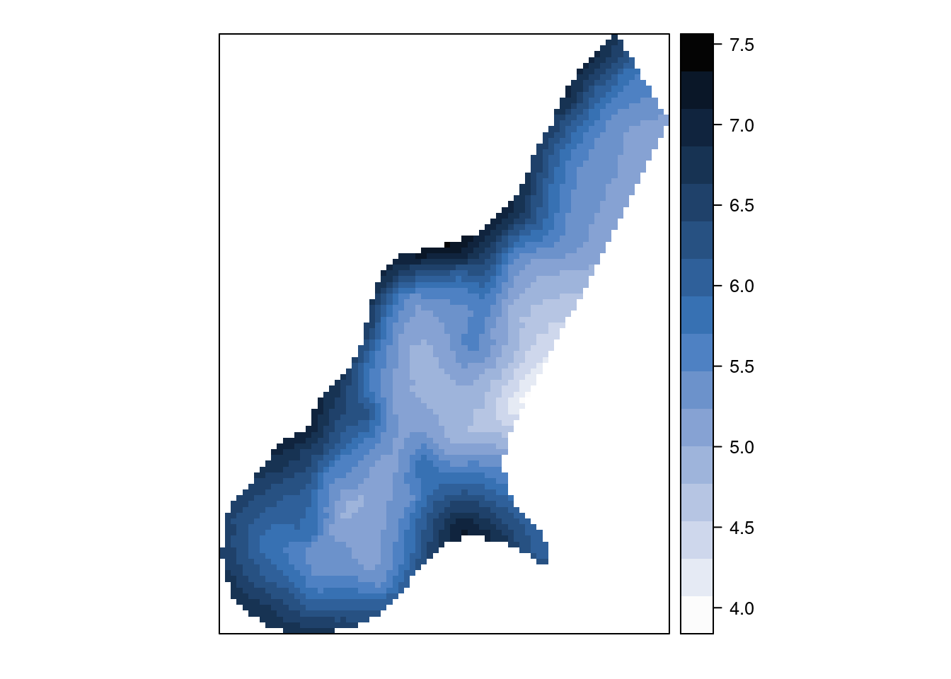
Figure 7.8: Concentration of zinc (log-scale) estimated with universal kriging for the meuse dataset.
7.3.3 Spatial Models using Stochastic Partial Differential Equations
Continuous spatial processes using a Matérn covariance function can be easily
fitted with INLA. Lindgren, Rue, and Lindström (2011) note that a spatial process with a
Matérn covariance can be obtained as the weak solution to a stochastic partial
differential equation (SPDE). Hence, they provide a solution to the equation
and they are able to work with a sparse representation of the solution that
fits within the INLA framework.
The solution \(u(s)\) can be represented as:
\[ u(s) = \sum_{k=1}^K \psi_k(s)w_k,\ s\in\mathcal{D} \]
In the previous equation, \(\{\psi_k(s)\}_{k=1}^K\) is a basis of functions needed to approximate the solution and \(w_k\) are associate coefficients, which are assumed to have a Gaussian distribution.
This spatial model is implemented as the spde latent effect in INLA.
However, defining this model to be used with INLA requires more work than
previous spatial models. In particular, a mesh needs to be defined over the
study region and it will be used to compute the approximation to the solution
(i.e., the spatial process). Krainski et al. (2018) describe SPDE models in detail,
but here we will summarize the different steps require to fit these models.
As a previous step, the boundary of the study region needs to be defined.
For this, the boundaries of the pixels in the meuse.grid will be
joined into a single region. This will provide a reasonable approximation
to the boundary of the study region.
#Boundary
meuse.bdy <- unionSpatialPolygons(
  as(meuse.grid, "SpatialPolygons"), rep (1, length(meuse.grid))
)
Next, a two-dimensional mesh will be defined to define the set of basis
functions using function inla.mesh.2d(). This will take the boundary of the
study region, as well as the dimensions of the maximum edge of the triangles
in the mesh and the length of the inner and outer offset.
#Define mesh
pts <- meuse.bdy@polygons[[1]]@Polygons[[1]]@coords
mesh <- inla.mesh.2d(loc.domain = pts, max.edge = c(150, 500),
  offset = c(100, 250) )
Figure 7.9 displays the boundary of the study region and the mesh created to approximate the solution of the SPDE to obtain the spatial model. A thick line separates the outer offset from the inner offset and the boundary of the study region. The figure has been obtained with the following code:
This triangulation defines the basis of functions that will be used to approximate the spatial process with Matérn covariance. In particular, the basis of functions is defined such as each function is one at a given vertex and zero outside the triangles that meet at that vertex. Hence, the functions have a compact support and they decay linearly from the vertex (where the value is 1) to the the boundary of the support (where it takes a value of zero). This means that for any given triangle in the mesh, only three functions in the basis will have non-zero values, which simplifies the computation of the estimates of the random effect at any given point because its estimate will be a linear combination of only three functions in the basis. See Chapter 2 in Krainski et al. (2018) for full details on how the basis functions are defined].
par(mar = c(0, 0, 0, 0))
plot(mesh, asp = 1, main = "")
lines(pts, col = 3, with = 2)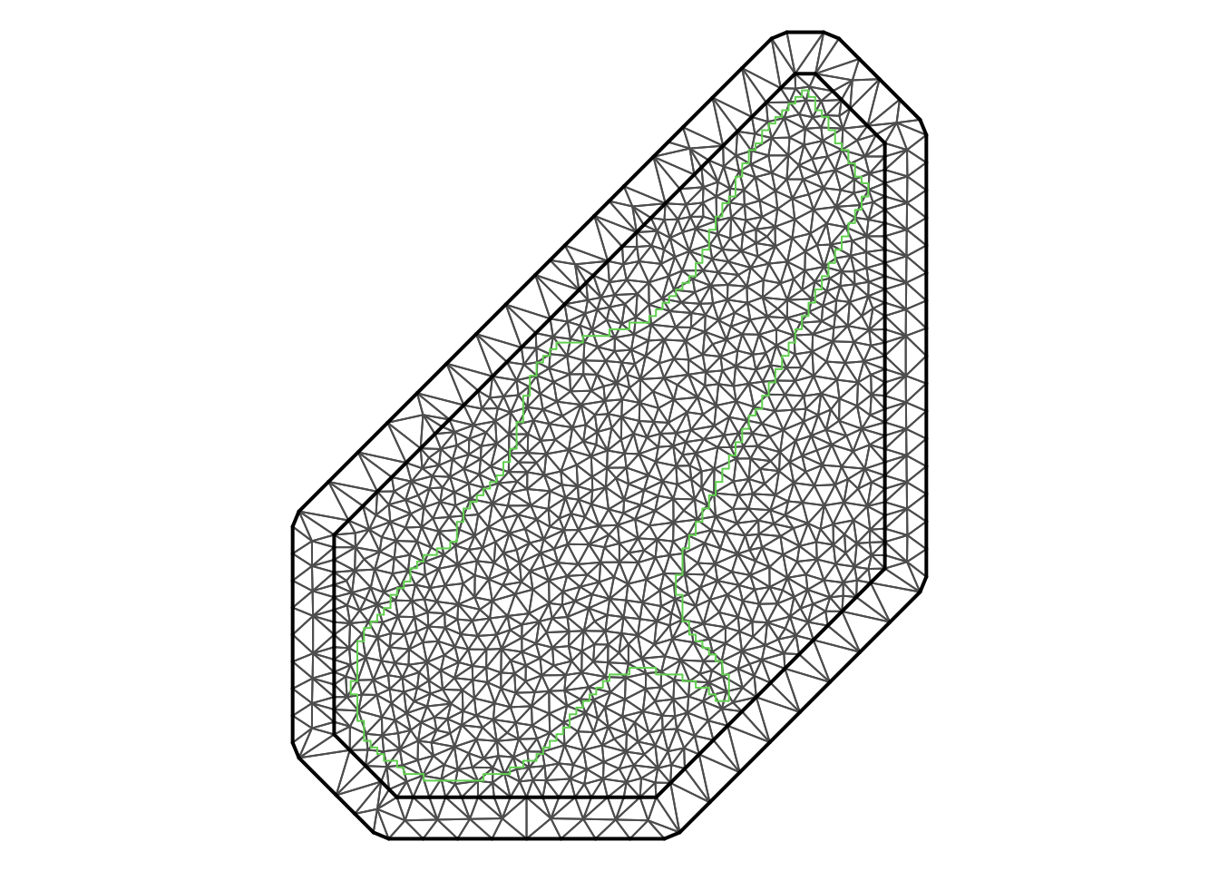
Figure 7.9: Mesh created for the analysis of the meuse dataset with INLA and SPDEs.
Function inla.spde2.matern() is used next to create an object for a Matérn
model. Furthermore, inla.spde.make.A is also used to create the projector
matrix \(A\) to map the projection of the SPDE to the observed points and
inla.spde.make.index a necessary list of named index vectors for the SPDE
model.
#Create SPDE
meuse.spde <- inla.spde2.matern(mesh = mesh, alpha = 2)
A.meuse <- inla.spde.make.A(mesh = mesh, loc = coordinates(meuse))
s.index <- inla.spde.make.index(name = "spatial.field",
  n.spde = meuse.spde$n.spde)
The previous steps will define how the solution to the SPDE that defined
the spatial process with a Matérn covariance is computed. This will
be used later when defining the spatial random effect using the f()
function in the formula that defines the INLA model.
Data passed to inla() when a SPDE is used needs to be in a particular format.
For this, the inla.stack function is provided. It will take data in different
ways, including the SPDE indices, and arrange them conveniently for model
fitting. In short, inla.stack will be a list with the following named
elements:
data: a list with data vectors.A: a list of projector matrices.effects: a list of effects (e.g., the SPDE index) or predictors (i.e., covariates).tag: a character with a label for this group of data.
For example, in order to define the data to be used for model fitting, we could do the following:
#Create data structure
meuse.stack <- inla.stack(data  = list(zinc = meuse$zinc),
  A = list(A.meuse, 1),
  effects = list(c(s.index, list(Intercept = 1)),
    list(dist = meuse$dist)),
  tag = "meuse.data")
Here, data is simply a list with a vector of the values of zinc. A is a
list with projector matrix A.meuse (used in the spatial model) and the value
\(1\). These two elements are associated with the two elements in effects, which
is a list of some information about the definition of the SPDE and some effects
with covariate dist. Finally, tag is a label to indicate that this
is the data in the meuse dataset.
This is all that is required to fit the model with an intercept, a covariate (distance to the river) plus the spatial random effect defined with a SPDE. However, given that we are studying a continuous spatial process, obtaining an estimate of the variable of interest (and the underlying spatial effect) in the study region is of interest.
For this reason, another stack of data can be defined for prediction. In this
case, the values of the response variable will be set to NA and the
predictive distributions computed. In addition, a different projector matrix
will be required in order to map the estimates of the spatial process to the
prediction points. This can be done using function inla.spde.make.A as before
using the points in the grid.
#Create data structure for prediction
A.pred <- inla.spde.make.A(mesh = mesh, loc = coordinates(meuse.grid))
meuse.stack.pred <- inla.stack(data = list(zinc = NA),
  A = list(A.pred, 1),
  effects = list(c(s.index, list (Intercept = 1)),
    list(dist = meuse.grid$dist)),
  tag = "meuse.pred")
Note that now a different tag ("meuse.pred") has been used in order to
be able to identify this part of the data in the stack to retrieve the
fitted values and other quantities of interest at the grid points.
Finally, both stacks of data can be put together into a single object with
inla.stack again. The resulting object will be the one passed to function
inla when fitting the model.
#Join stack
join.stack <- inla.stack(meuse.stack, meuse.stack.pred)
To define the model that will be fitted, the spatial effects need to be added
using the f() function. The index passed to this function will be the one
created before with inla.spde.make.index and whose name is spatial.field.
In addition, the model will be of type spde.
#Fit model
form <- log(zinc) ~ -1 + Intercept + dist + f(spatial.field, model = spde)
Data passed to the inla function needs to be joined with the
definition of the SPDE to fit the spatial model. This is done
with function inla.stack.data. Furthermore, control.predictor will
need to take the projector matrix for the whole dataset (model fitting
and prediction) using function inla.stack.A in join.stack.
m1 <- inla(form, data = inla.stack.data(join.stack, spde = meuse.spde),
  family = "gaussian",
  control.predictor = list(A = inla.stack.A(join.stack), compute = TRUE),
  control.compute = list(cpo = TRUE, dic = TRUE))

#Summary of results
summary(m1)
##
## Call:
## c("inla(formula = form, family = \"gaussian\", data =
## inla.stack.data(join.stack, ", " spde = meuse.spde),
## control.compute = list(cpo = TRUE, dic = TRUE), ", "
## control.predictor = list(A = inla.stack.A(join.stack), compute =
## TRUE))" )
## Time used:
## Pre = 0.405, Running = 66.9, Post = 0.519, Total = 67.8
## Fixed effects:
## mean sd 0.025quant 0.5quant 0.975quant mode kld
## Intercept 6.591 0.143 6.317 6.588 6.889 6.581 0
## dist -2.808 0.380 -3.563 -2.807 -2.058 -2.805 0
##
## Random effects:
## Name Model
## spatial.field SPDE2 model
##
## Model hyperparameters:
## mean sd 0.025quant 0.5quant
## Precision for the Gaussian observations 18.72 6.437 8.97 17.79
## Theta1 for spatial.field 4.41 0.299 3.83 4.40
## Theta2 for spatial.field -4.94 0.309 -5.57 -4.94
## 0.975quant mode
## Precision for the Gaussian observations 33.94 16.02
## Theta1 for spatial.field 5.01 4.38
## Theta2 for spatial.field -4.36 -4.91
##
## Expected number of effective parameters(stdev): 88.80(17.55)
## Number of equivalent replicates : 1.75
##
## Deviance Information Criterion (DIC) ...............: 80.44
## Deviance Information Criterion (DIC, saturated) ....: 245.01
## Effective number of parameters .....................: 87.41
##
## Marginal log-Likelihood: -108.15
## CPO and PIT are computed
##
## Posterior marginals for the linear predictor and
## the fitted values are computedAccording to the model fitted there is a clear reduction in the concentration of zinc as distance to the river increases. This is consistent with previous findings and the results from the universal kriging.
Obtaining the fitted values at the prediction points requires first getting the
index for the points in the meuse.pred part of the stack. This can be
easily done with function inla.stack.index (see code below). Similarly,
fitted values for the meuse.data can be obtained. Next, the index is used to
obtain the posterior means and other summary statistics computed on the
predictive distributions and these added to the meuse.grid object for
plotting.
#Get predicted data on grid
index.pred <- inla.stack.index(join.stack, "meuse.pred")$data

meuse.grid$zinc.spde <- m1$summary.fitted.values[index.pred, "mean"]
meuse.grid$zinc.spde.sd <- m1$summary.fitted.values[index.pred, "sd"]
Figure 7.10 shows the posterior means of the concentrations of zinc in the log-scale and Figure 7.11 the prediction standard deviations, which are a measure of the uncertainty about the predictions. Point estimates of the concentration seem to be very similar between universal kriging and the model fitted with INLA. However, prediction uncertainty seems to be smaller with the SPDE model. Note that here we are comparing results from two different inference methods. Furthermore, these differences in the uncertainty may be due to the different ways in which the covariance of the spatial effect is computed and a shrinkage effect due to the priors in the Bayesian model.
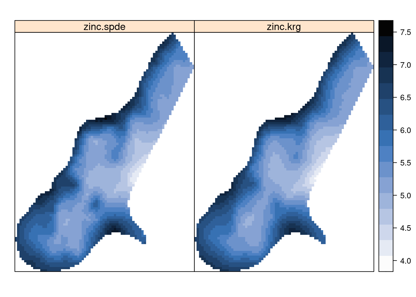
Figure 7.10: Posterior means of log-concentration of zinc.
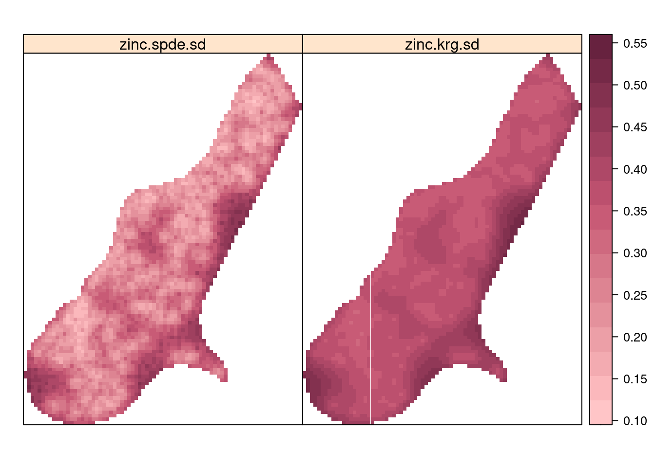
Figure 7.11: Posterior prediction standard deviations of log-concentration of zinc.
Besides the estimation of the concentration of zinc, studying the underlying
spatial process may be of interest. For this reason, it is important
to study the estimates of the parameters of the spatial effect. INLA
reports summary estimates of the parameters in the internal scale, but
the marginals of the variance and range parameters can be obtained
using function inla.spde2.result. Then, summary statistics on the parameters
using their respective posterior marginals can be computed with function
inla.zmarginal.
#Compute statistics in terms or range and variance
spde.est <- inla.spde2.result(inla = m1, name = "spatial.field",
  spde = meuse.spde, do.transf = TRUE)

#Kappa
#inla.zmarginal(spde.est$marginals.kappa[[1]])
#Variance
inla.zmarginal(spde.est$marginals.variance.nominal[[1]])
## Mean 0.243931
## Stdev 0.0578992
## Quantile 0.025 0.152402
## Quantile 0.25 0.202374
## Quantile 0.5 0.236094
## Quantile 0.75 0.27715
## Quantile 0.975 0.378597#Range
inla.zmarginal(spde.est$marginals.range.nominal[[1]])## Mean 416.358
## Stdev 132.805
## Quantile 0.025 221.148
## Quantile 0.25 321.188
## Quantile 0.5 393.715
## Quantile 0.75 487.098
## Quantile 0.975 737.859A similar summary for the variogram used in the universal kriging can be obtained as follows:
#Summary stats; nugget is a 'random' effect with a variance
fit.vgm
## model psill range
## 1 Nug 0.07643 0.0
## 2 Sph 0.20529 728.7The sill and range of the variogram are very similar to the estimates obtained for the Matérn covariance computed using SPDE. The nugget effect in the variogram can be regarded as a measurement error or the variance in the Gaussian likelihood. A rough comparison can be done between the sill of the nugget effect in the variogram and the inverse of the mode of the precision of the Gaussian likelihood:
#Precision of nugget term (similar to precision of error term)
1 / fit.vgm$psill[1]
## [1] 13.08The resulting value is very similar to the posterior mean of the precision of the Gaussian likelihood. Hence, both universal kriging and the SPDE model provide similar estimates of the underlying spatial process.
As a final remark, it is worth mentioning that the inlabru package
(Bachl et al. 2019) can simplify the way in which the model is defined and fit.
Furthermore, the meshbuilder() function in the INLA package can help to
define and assess the adequacy of a mesh in an interactive way
(Krainski et al. 2018).
7.4 Point patterns
In Section 7.2 we considered the analysis of a point pattern using a discrete representation of the process. However, point patterns can also be studied as a continuous process. In particular, we will consider inhomogeneous Poisson point processes defined by a given intensity \(\lambda(x)\) which varies spatially and may also be modulated by some covariates.
Hence, the intensity can be represented as
\[ \lambda (x) = \lambda_0(x) \exp(\mathbf{\beta} \mathbf{x}) \]
Here, \(\lambda_0(x)\) is an underlying spatial distribution modulated by a vector of covariates \(\mathbf{x}\) with associated coefficients \(\mathbf{\beta}\).
The intensity can be estimated semi-parametrically by using a non-parametric estimate of \(\lambda_0(x)\) (Diggle 2013). For example, Diggle et al. (2007) use kernel smoothing to estimate \(\lambda_0(x)\) and a logistic regression (conditional of the locations of the observed events) to obtain estimates of the vector of coefficients \(\mathbf{\beta}\). Below we will show how to model \(\log(\lambda(x))\) using a Gaussian process to define a log-Gaussian Cox process (Krainski et al. 2018).
7.4.1 Log-Gaussian Cox processes
Simpson et al. (2016) describe the use of SPDE to estimate \(\lambda(x)\) using log-Gaussian Cox models. In particular, \(\lambda_0(x)\) is estimated using a SPDE, i.e.,
\[ \log(\lambda_0(x)) = S(x) \]
Here, \(S(x)\) is a stationary and isotropic Gaussian spatial process with a Matérn covariance. This spatial process can be estimated using the SPDE approach described in Section 7.3.
Simpson et al. (2016) show how fitting the previous model is similar to fitting a Poisson process on an extended data set using the locations of the events and the integration points of the SPDE mesh. This extended dataset needs to be created as follows:
The value of the response is 0 at the integration points and 1 at the observed points.
Each data point will have an associated weight, which will be 0 for the observed data and the area of its associated polygon in a Voronoi tessellation using the integration points.
Weights required to estimate the model (see below).
The inlabru package (Bachl et al. 2019) provides a simple interface for the
analysis of point patterns with INLA and SPDE models. However, we provide here
full details on the whole process to fit the model according to
Simpson et al. (2016). The construction of the expanded dataset as well as the
steps required for model fitting are described in the next example.
The meshbuilder() function in the INLA package can also be used to test
the adequacy of the mesh created for a SPDE latent effect (see also Krainski et al. 2018).
7.4.2 Castilla-La Mancha forest fires
The clmfires dataset in the spatstat package records the occurrence of
forest fires in the region of Castilla-La Mancha (Spain) from 1998 to 2007.
This dataset has been put together by Prof. Jorge Mateu. and Table
7.7 provides a summary of the variables in the dataset.
| Variable | Description |
|---|---|
cause |
Cause of the fire (lightning, accident, intentional or other) |
burnt.area |
Total area burned (in hectares) |
date |
Date of fire |
julian.date |
Date of fire, as days elapsed since 1 January 1998 |
Furthermore, the clmfires.extra dataset contains two objects with covariate
information for the study region. These two objects are named clmcov100 and
clmcov200 because they provide the information in several im objects (that
represents raster data in the spatstat package) in a raster of size 100x100
and 200x200 pixels, respectively. Each one is a named list of four im objects
with the variables in Table 7.8. Covariate landuse is a
factor with levels: ‘urban’, ‘farm’ (which includes farms and orchards),
‘meadow’, ‘denseforest’, ‘conifer’ (which includes conifer forests and
plantations), ‘mixedforest’, ‘grassland’, ‘bush’, ‘scrub’ and ‘artifgreen’
(such as golf courts).
| Variable | Description |
|---|---|
elevation |
Elevation of the terrain (in meters). |
orientation |
Orientation of the terrain (in degrees). |
slope |
Slope. |
landuse |
Land use (a factor, see text for details). |
First of all, the data will be loaded and the observed points in the period 2004 to 2007 selected. This is done because of the concern about how the location of the fires was done prior to 2004.
library("spatstat")
data(clmfires)

#Subset to 2004 to 2007
clmfires0407 <- clmfires[clmfires$marks$date >= "2004-01-01"]
Next, given that the pixels classified as artifgreen are just a few,
we have merged this category with urban (because both are human-built):
# Set `urban` instead of `artifgreen`
idx <- which(clmfires.extra$clmcov100$landuse$v %in% c("artifgreen",
  "farm"))
clmfires.extra$clmcov100$landuse$v[idx] <- "urban"

# Convert to factor
clmfires.extra$clmcov100$landuse$v <-
factor(as.character(clmfires.extra$clmcov100$landuse$v))
# Set right dimension of raster object

dim(clmfires.extra$clmcov100$landuse$v) <- c(100, 100)
Note that the reference category now is bush so the effects of all the other
levels will be relative to this category (unless the intercept is removed from
the model):
clmfires.extra$clmcov100$landuse## factor-valued pixel image
## factor levels:
## [1] "bush" "conifer" "denseforest" "grassland" "meadow"
## [6] "mixedforest" "scrub" "urban"
## 100 x 100 pixel array (ny, nx)
## enclosing rectangle: [-2.1, 397.9] x [-2.1, 397.9] kilometresCovariates elevation and orientation are rescaled so that they
are expressed in kilometers and radians. This is done in order to avoid
problems when fitting the spatial model with INLA. This is particularly
important for elevation because it is originally in meters.
#In addition, we will rescale `elevation` (to express it in kilometers) and
#`orientation` (to be in radians) so that fixed effects are better estimated:
clmfires.extra$clmcov100$elevation <-
  clmfires.extra$clmcov100$elevation / 1000
clmfires.extra$clmcov100$orientation <-
  clmfires.extra$clmcov100$orientation * pi / 180
Juan, Mateu, and Díaz-Avalos (2010) provide an analysis of the forest fires in 1998 alone and they suggest analyzing this type of data using log-Gaussian Cox processes. In addition, they show that forest fires due to lightning have a different pattern. Hence, we will focus our analysis of these type of fires and subset these points from the original dataset:
clmfires0407 <- clmfires0407[clmfires0407$marks$cause == "lightning", ]Figure 7.12 shows the boundary of Castilla-La Mancha and the location of the forest fires due to lightning. Note how most of them appear in the east part of the region.
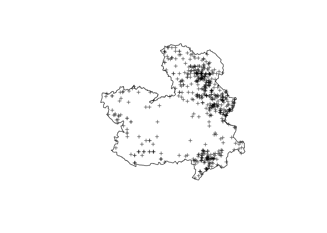
Figure 7.12: Location of forest fires due to a lightning in Castilla-La Mancha in the period.
Next, the boundary of the study region will be extracted from the ppp object
and it will be used to create a mesh over the study region. This mesh will
be used to estimate the latent stationary and isotropic Gaussian process
with Matérn covariance using the SPDE approach in INLA.
clm.bdy <- do.call(cbind, clmfires0407$window$bdry[[1]])
#Define mesh
clm.mesh <- inla.mesh.2d(loc.domain = clm.bdy, max.edge = c(15, 50),
  offset = c(10, 10))
As discussed before, model fitting requires an expanded dataset with the locations of the forest fires and the integration points in the mesh.
#Points
clm.pts <- as.matrix(coords(clmfires0407))
clm.mesh.pts <- as.matrix(clm.mesh$loc[, 1:2])
allpts <- rbind(clm.mesh.pts, clm.pts)

# Number of vertices in the mesh
nv <- clm.mesh$n
# Number of points in the data
n <- nrow(clm.pts)
Next, the SPDE latent effect needs to be defined. In this case, penalized complexity priors (see Section 5.4) are used for the range and standard deviation of the Matérn covariance. In particular, the prior of the range \(r\) is set by defining \((r_0, p_r)\) such that
\[ P(r < r_0) = p_r. \]
Similarly, the penalized complexity prior for the standard deviation \(\sigma\) is defined by pair \((\sigma_0, p_s)\), such that
\[ P(\sigma >\sigma_0) = p_s. \]
As a prior assumption the probability of the range being higher than
50 is small (i.e., \(r_0 = 50\) and \(p_r=0.9\)) and that the probability of
\(\sigma\) being higher than 5 is also small (i.e., \(\sigma_0=1\) and
\(p_s = 0.01\)). A SPDE latent effect with this type of prior is created
with function inla.spde2.pcmatern() as follows:
#Create SPDE
clm.spde <- inla.spde2.pcmatern(mesh = clm.mesh, alpha = 2,
  prior.range = c(50, 0.9), # P(range < 50) = 0.9
  prior.sigma = c(1, 0.01) # P(sigma > 10) = 0.01
)
See also Sørbye et al. (2019) for some comments on setting priors when fitting log-Gaussian Cox processes to point patterns using SPDEs.
The weights associated with the mesh points are equal to the
area of the surrounding polygon in a Voronoi tessellation that
falls inside the study region. This is
computed below using packages deldir (Turner 2019), rgeos (R. Bivand and Rundel 2019)
and SDraw (McDonald and McDonald 2019). Note that spatial data must be in one of the
objects in the sp package and, for this reason, the boundary
is converted into a SpatialPolygons object and function voronoi.polygons()
is used as it returns the Voronoi tessellation as a SpatialPolygons object
as well.
library("deldir")
library("SDraw")

# Voronoi polygons (as SpatialPolygons)
mytiles <- voronoi.polygons(SpatialPoints(clm.mesh$loc[, 1:2]))

# C-LM bounday as SpatialPolygons
clmbdy.sp <- SpatialPolygons(list(Polygons(list(Polygon (clm.bdy)),
  ID = "1")))

#Compute weights
require(rgeos)

w <- sapply(1:length(mytiles), function(p) {
  aux <- mytiles[p, ]

  if(gIntersects(aux, clmbdy.sp) ) {
    return(gArea(gIntersection(aux, clmbdy.sp)))
  } else {
    return(0)
  }
})
Note how the sum of the weights is equal to the area of the study region:
# Sum of weights
sum(w)
## [1] 79355# Area of study region
gArea(clmbdy.sp)## [1] 79355Figure 7.13 shows the mesh points (black dots) as well as the resulting Voronoi tessellation and the boundary of Castilla-La Mancha. The weight associated with each point is the area of the associated Voronoi polygon inside the region of Castilla-La Mancha.
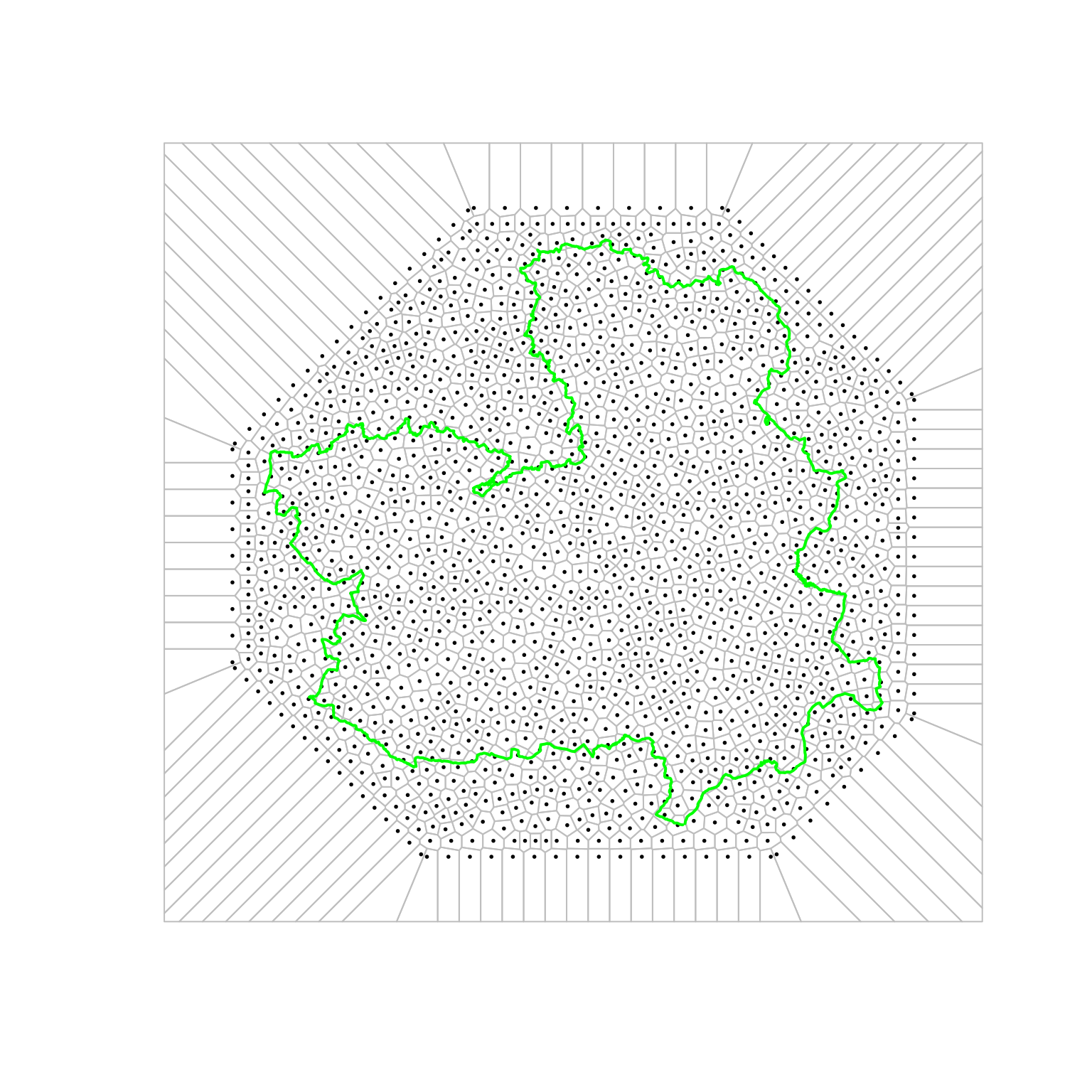
Figure 7.13: Voronoi tesselletation used in the analysis of forest fires in Castilla-La Mancha.
Once the weights associated with the mesh points have been computed,
the expanded dataset can be put together. Values of the covariates at
the integration points are required to fit the model. These are
obtained from the raster data available in the clmfires.extra dataset.
#Prepare data
y.pp = rep(0:1, c(nv, n))
e.pp = c(w, rep(0, n))

lmat <- inla.spde.make.A(clm.mesh, clm.pts)
imat <- Diagonal(nv, rep(1, nv))

A.pp <-rbind(imat, lmat)

clm.spde.index <- inla.spde.make.index(name = "spatial.field",
  n.spde = clm.spde$n.spde)
Covariates required in the analysis are obtained by using different functions
in the spatstat package. In particular, function nearest.pixel() is
used below to assign to each point (in the expanded dataset) the values of the covariates of the nearest pixel in the raster object.
#Covariates
allpts.ppp <- ppp(allpts[, 1], allpts[, 2], owin(xrange = c(-15.87, 411.38),
  yrange = c(-1.44, 405.19)))

# Assign values of covariates to points using value of nearest pixel
covs100 <- lapply(clmfires.extra$clmcov100, function(X){
  pixels <- nearest.pixel(allpts.ppp$x, allpts.ppp$y, X)
  sapply(1:npoints(allpts.ppp), function(i) {
    X[pixels$row[i], pixels$col[i]]
  })
})

# Intercept for spatial model
covs100$b0 <- rep(1, nv + n)
Once all the required data have been obtained, the data stack for model fitting is created:
#Create data structure
clm.stack <- inla.stack(data = list(y = y.pp, e = e.pp),
  A = list(A.pp, 1),
  effects = list(clm.spde.index, covs100),
  tag = "pp")
Similarly, another stack of data will be put together for prediction. This will
require the locations of the points in a regular grid as well as the values of
the covariates at the grid points (now using the subsetting operator in the
spatstat package). The grid used will be the same as the one
used in the raster data with the covariates.
#Data structure for prediction
library("maptools")
sgdf <- as(clmfires.extra$clmcov100$elevation, "SpatialGridDataFrame")
sp.bdy <- as(clmfires$window, "SpatialPolygons")
idx <- over(sgdf, sp.bdy)
spdf <- as(sgdf[!is.na(idx), ], "SpatialPixelsDataFrame")

pts.pred <- coordinates(spdf)
n.pred <- nrow(pts.pred)

#Get covariates (using subsetting operator in spatstat)
ppp.pred <- ppp(pts.pred[, 1], pts.pred[, 2], window = clmfires0407$window)
covs100.pred <- lapply(clmfires.extra$clmcov100, function(X) {
  X[ppp.pred]
})

# Intercept for spatial model
covs100.pred$b0 <- rep(1, n.pred)

#Prediction points
A.pred <- inla.spde.make.A (mesh = clm.mesh, loc = pts.pred)
clm.stack.pred <- inla.stack(data = list(y = NA),
   A = list(A.pred, 1),
   effects = list(clm.spde.index, covs100.pred),
   tag = "pred")
Finally, all data stacks will be put together into a single object:
#Join data
join.stack <- inla.stack(clm.stack, clm.stack.pred)
Model fitting will be carried out similarly as in the geostatistics case.
However, now the likelihood to be used in a Poisson and the weights associated
to the points in the expanded dataset need to be passed using parameter E.
The integration strategy is set to "eb" in order to reduce computation
time (Krainski et al. 2018).
The first model estimates the intensity of the point process using an intercept and the SPDE latent effect. This estimate should be similar to a kernel density smoothing (Gómez-Rubio, Cameletti, and Finazzi 2015).
pp.res0 <- inla(y ~ 1 +
    f(spatial.field, model = clm.spde),
  family = "poisson", data = inla.stack.data(join.stack),
  control.predictor = list(A = inla.stack.A(join.stack), compute = TRUE,
    link = 1),
  control.inla = list(int.strategy = "eb"),
  E = inla.stack.data(join.stack)$e)
Next, the model is defined to include covariates and the SPDE latent effect.
pp.res <- inla(y ~ 1 + landuse + elevation + orientation + slope +
    f(spatial.field, model = clm.spde),
  family = "poisson", data = inla.stack.data(join.stack),
  control.predictor = list(A = inla.stack.A(join.stack), compute = TRUE,
    link = 1), verbose = TRUE,
  control.inla = list(int.strategy = "eb"),
E = inla.stack.data(join.stack)$e)summary(pp.res)##
## Call:
## c("inla(formula = y ~ 1 + landuse + elevation + orientation +
## slope + ", " f(spatial.field, model = clm.spde), family =
## \"poisson\", data = inla.stack.data(join.stack), ", " E =
## inla.stack.data(join.stack)$e, verbose = TRUE, control.predictor =
## list(A = inla.stack.A(join.stack), ", " compute = TRUE, link = 1),
## control.inla = list(int.strategy = \"eb\"))" )
## Time used:
## Pre = 0.801, Running = 75.3, Post = 1.2, Total = 77.3
## Fixed effects:
## mean sd 0.025quant 0.5quant 0.975quant mode kld
## (Intercept) -2.845 0.304 -3.441 -2.845 -2.249 -2.845 0
## landuseconifer 0.051 0.209 -0.360 0.051 0.462 0.051 0
## landusedenseforest 0.517 0.256 0.007 0.519 1.014 0.523 0
## landusegrassland 0.222 0.237 -0.247 0.223 0.683 0.226 0
## landusemeadow 0.279 0.344 -0.416 0.286 0.936 0.300 0
## landusemixedforest 0.750 0.246 0.265 0.751 1.231 0.752 0
## landusescrub 0.386 0.199 -0.004 0.385 0.777 0.385 0
## landuseurban 0.211 0.182 -0.142 0.209 0.573 0.206 0
## elevation 0.117 0.348 -0.569 0.119 0.795 0.121 0
## orientation -0.020 0.029 -0.077 -0.020 0.037 -0.020 0
## slope -0.017 0.009 -0.036 -0.017 0.001 -0.017 0
##
## Random effects:
## Name Model
## spatial.field SPDE2 model
##
## Model hyperparameters:
## mean sd 0.025quant 0.5quant 0.975quant
## Range for spatial.field 120.58 22.767 84.255 117.61 173.22
## Stdev for spatial.field 1.27 0.185 0.957 1.25 1.68
## mode
## Range for spatial.field 111.32
## Stdev for spatial.field 1.21
##
## Expected number of effective parameters(stdev): 101.90(0.00)
## Number of equivalent replicates : 21.35
##
## Marginal log-Likelihood: -3072.82
## Posterior marginals for the linear predictor and
## the fitted values are computedThe summary of the model with covariates provides some insight on the factors
associated to the location of forest fires in this region. Elevation,
orientation and slope do not seem to have an effect. Regarding land use,
bush is the baseline and it does not seem that there are differences with
most of the different types of land use. However, dense and mixed forest (and,
perhaps, scrub) seem to have an increased number of forest fires due to
lightning as compared to the baseline level.
The fitted values of the intensity with both models can be retrieved from the
model fits and added to the SpatialPixelsDataFrame with the data to
be plotted:
#Prediction
idx <- inla.stack.index(join.stack, 'pred')$data
# MOdel with no covariates
spdf$SPDE0 <- pp.res0$summary.fitted.values[idx, "mean"]
#Model with covariates
spdf$SPDE <- pp.res$summary.fitted.values[idx, "mean"]
Figure 7.14 displays the posterior means of the estimated intensity at the grid points for both models and it can be used to assess fire risk. For example, a region of high risk can be found in the southeast part of Castilla-La Mancha (municipalities of Yeste, Letur and Nerpio).
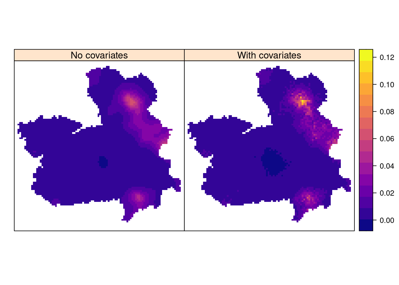
Figure 7.14: Intensity of forest fires in Castilla-La Mancha (Spain). The region is about 400 x 400 km.
In order to understand the latent spatial pattern, the marginals of its parameters can be estimated similarly as in the geostatistics example:
#Compute statistics in terms or range and variance
spde.clm.est <- inla.spde2.result(inla = pp.res, name = "spatial.field",
  spde = clm.spde, do.transf = TRUE)

#Variance
inla.zmarginal(spde.clm.est$marginals.variance.nominal[[1]])
## Mean 1.6395
## Stdev 0.486537
## Quantile 0.025 0.918128
## Quantile 0.25 1.29075
## Quantile 0.5 1.5578
## Quantile 0.75 1.90123
## Quantile 0.975 2.81266#Range
inla.zmarginal(spde.clm.est$marginals.range.nominal[[1]])## Mean 120.544
## Stdev 22.5798
## Quantile 0.025 84.384
## Quantile 0.25 104.34
## Quantile 0.5 117.562
## Quantile 0.75 133.71
## Quantile 0.975 172.63Note that the output from the model already provided summary statistics for the range and variance of the spatial process. According to the value of the spatial range, it seems that the spatial random effect accounts for medium-scale spatial variation (remember that the region covers an area of about 400 x 400 km). The estimate of the spatial variance seems to be small, which makes the spatial variation not have too extreme peaks.
References
Bachl, Fabian E., Finn Lindgren, David L. Borchers, and Janine B. Illian. 2019. “inlabru: An R Package for Bayesian Spatial Modelling from Ecological Survey Data.” Methods in Ecology and Evolution 10: 760–66. https://doi.org/10.1111/2041-210X.13168.
Baddeley, Adrian, Ege Rubak, and Rolf Turner. 2015. Spatial Point Patterns: Methodology and Applications with R. London: Chapman; Hall/CRC Press. http://www.crcpress.com/Spatial-Point-Patterns-Methodology-and-Applications-with-R/Baddeley-Rubak-Turner/9781482210200/.
Banerjee, S., B. P. Carlin, and A. E. Gelfand. 2014. Hierarchical Modeling and Analysis for Spatial Data. 2nd ed. Boca Raton, FL: Chapman & Hall/CRC.
Bivand, Roger, and Colin Rundel. 2019. Rgeos: Interface to Geometry Engine - Open Source (’Geos’). https://CRAN.R-project.org/package=rgeos.
Bivand, Roger S. 2017. “Revisiting the Boston Data Set - Changing the Units of Observation Affects Estimated Willingness to Pay for Clean Air.” REGION 1 (4): 109–27. http://openjournals.wu.ac.at/ojs/index.php/region/article/view/107.
Bivand, Roger S., Virgilio Gómez-Rubio, and Håvard Rue. 2015. “Spatial Data Analysis with R-INLA with Some Extensions.” Journal of Statistical Software 63 (20): 1–31. http://www.jstatsoft.org/v63/i20/.
Bivand, Roger S., Edzer Pebesma, and Virgilio Gómez-Rubio. 2013. Applied Spatial Data Analysis with R. 2nd ed. New York: Springer.
Bivand, Roger, and David W. S. Wong. 2018. “Comparing Implementations of Global and Local Indicators of Spatial Association.” TEST 27 (3): 716–48. https://doi.org/10.1007/s11749-018-0599-x.
Blangiardo, Marta, and Michela Cameletti. 2015. Spatial and Spatio-Temporal Bayesian Models with R-INLA. Chichester, UK: John Wiley & Sons Ltd.
Condit, R. 1998. Tropical Forest Census Plots. Springer-Verlag Berlin Heidelberg.
Condit, R., S. P. Hubbell, and R. B. Foster. 1996. “Changes in Tree Species Abundance in a Neotropical Forest: Impact of Climate Change.” Journal of Tropical Ecology 12: 231–56.
Cressie, Noel. 2015. Statistics for Spatial Data. Revised. Hoboken, New Jersey: John Wiley & Sons, Inc.
Cressie, Noel, and Christopher K. Wikle. 2011. Statistics for Spatio-Temporal Data. Hoboken, New Jersey: John Wiley & Sons, Inc.
Diggle, Peter J. 2013. Statistical Analysis of Spatial and Spatio-Temporal Point Patterns. 3rd ed. Chapman; Hall/CRC Press.
Diggle, Peter J., Virgilio Gómez‐Rubio, Patrick E. Brown, Amanda G. Chetwynd, and Susan Gooding. 2007. “Second‐Order Analysis of Inhomogeneous Spatial Point Processes Using Case–Control Data.” Biometrics 2 (63): 550–57.
Gilley, O. W., and R. Kelley Pace. 1996. “On the Harrison and Rubinfeld Data.” Journal of Environmental Economics and Management 31: 403–5.
Gómez-Rubio, Virgilio, Michela Cameletti, and Francesco Finazzi. 2015. “Analysis of Massive Marked Point Patterns with Stochastic Partial Differential Equations.” Spatial Statistics 14: 179–96. https://doi.org/https://doi.org/10.1016/j.spasta.2015.06.003.
Harrison, David, and Daniel L. Rubinfeld. 1978. “Hedonic Housing Prices and the Demand for Clean Air.” Journal of Environmental Economics and Management 5: 81–102.
Hubbell, S. P., and R. B. Foster. 1983. “Diversity of Canopy Trees in a Neotropical Forest and Implications for Conservation.” In Tropical Rain Forest: Ecology and Management, edited by S. L. Sutton, T. C. Whitmore, and A. C. Chadwick, 25–41. Oxford: Blackwell Scientific Publications.
Juan, P., J. Mateu, and C. Díaz-Avalos. 2010. “Characterizing Spatial-Temporal Forest Fire Patterns.” In METMA V: International Workshop on Spatio-Temporal Modelling. Santiago de Compostela, Spain.
Krainski, Elias T., Virgilio Gómez-Rubio, Haakon Bakka, Amanda Lenzi, Daniela Castro-Camilo, Daniel Simpson, Finn Lindgren, and Håvard Rue. 2018. Advanced Spatial Modeling with Stochastic Partial Differential Equations Using R and INLA. Boca Raton, FL: Chapman & Hall/CRC.
Leroux, B., X. Lei, and N. Breslow. 1999. “Estimation of Disease Rates in Small Areas: A New Mixed Model for Spatial Dependence.” In Statistical Models in Epidemiology, the Environment and Clinical Trials, edited by M Halloran and D Berry, 135–78. New York: Springer-Verlag.
Lindgren, Finn, Håvard Rue, and Joham Lindström. 2011. “An Explicit Link Between Gaussian Fields and Gaussian Markov Random Fields: The Stochastic Partial Differential Equation Approach (with Discussion).” Journal of the Royal Statistical Society, Series B 73 (4): 423–98.
Lovelace, Robin, Jakub Nowosad, and Jannes Muenchow. 2019. Geocomputation with R. Boca Raton, FL: Chapman & Hall/CRC.
McDonald, Trent, and Aidan McDonald. 2019. SDraw: Spatially Balanced Samples of Spatial Objects. https://CRAN.R-project.org/package=SDraw.
Møller, J., and R. P. Waagepetersen. 2007. “Modern Spatial Point Process Modelling and Inference (with Discussion).” Scandinavian Journal of Statistics 34: 643–711.
Pebesma, E. J. 2004. “Multivariable Geostatistics in S: The Gstat Package.” Computers & Geosciences 30: 683–91.
Simpson, Daniel, Janine B. Illian, S. H. Sørbye, and Håvard Rue. 2016. “Going Off Grid: Computationally Efficient Inference for Log-Gaussian Cox Processes.” Biometrika 1 (103): 49–70.
Sørbye, Sigrunn H., Janine B. Illian, Daniel P. Simpson, David Burslem, and Håvard Rue. 2019. “Careful Prior Specification Avoids Incautious Inference for Log-Gaussian Cox Point Processes.” Journal of the Royal Statistical Society: Series C (Applied Statistics) 68 (3): 543–64. https://doi.org/10.1111/rssc.12321.
Turner, Rolf. 2019. Deldir: Delaunay Triangulation and Dirichlet (Voronoi) Tessellation. https://CRAN.R-project.org/package=deldir.
Ugarte, M. D., A. Adin, T. Goicoa, and A. F. Militino. 2014. “On Fitting Spatio-Temporal Disease Mapping Models Using Approximate Bayesian Inference.” Statistical Methods in Medical Research 23: 507–30. https://doi.org/10.1177/0962280214527528.