Chapter 5 Priors in R-INLA

5.1 Introduction

Priors play an important role in Bayesian analysis and their definition should be considered very carefully. In this chapter prior definition in INLA is described in more detail. If no prior distribution on a given parameter is set, a default one will be used. Hence, it is important to know what the default priors are, as well as other possible alternatives.

INLA provides different ways to define the prior of the hyperparameters, and all of them are covered in this chapter. First of all, there is a list of implemented priors available that can be used in the models straight away. These are described in Section 5.2. New priors can easily be implemented as well, as described in Section 5.3. The new Penalized Complexity priors, or PC-priors, are introduced in Section 5.4. Given that INLA can fit Bayesian models very fast, sensitivity analysis on the priors can be done, as seen in Section 5.5. Finally, scaling of the latent random effects and prior definition is tackled in Section 5.6.

5.2 Selection of priors

The first thing to know about setting priors in INLA is that priors are set in the internal representation of the parameter, which may be different from the scale of the parameter in the model. For example, precisions are represented in the internal scale in the log-scale. This is computationally convenient because in the internal scale the parameter is not bounded. For example, the posterior mode of the hyperparameters can be obtained by maximizing the sum of the log-likelihood and the log-prior on the hyperparameters. This optimization step is used by INLA at the beginning of the model fitting to locate the posterior mode of the hyperparameters and find the region of high posterior density.

Note that the internal representation of the hyperparameters is described in the documentation of the INLA package corresponding to the relevant likelihood or latent effect. Table 5.3 below summarizes the different internal representations for different hyperparameters.

In order to use one of the prior distributions implemented in INLA it is necessary to set them explicitly. Priors on the hyperparameters of the likelihood must be passed by defining argument hyper within control.family in the call to INLA. Priors on the hyperparameters of the latent effects are set using the parameter hyper, inside the f() function.

Parameter hyper is a named list so that each element in the list defines the prior for a different hyperparameter. The names used in the list can be the names of the parameters or those used for the internal representation. These can be checked in the documentation or using function inla.models(), as described in Section 2.3.2. The next example focuses on the iid latent effect, which only has the precision hyperparameter, and shows the name in the internal representation ("theta"), the name of the parameter ("log precision") and a short name ("prec"):

names(inla.models()$latent$iid$hyper)

## [1] "theta"

inla.models()$latent$iid$hyper$theta$name

## [1] "log precision"
## attr(,"inla.read.only")
## [1] FALSE

inla.models()$latent$iid$hyper$theta$short.name

## [1] "prec"
## attr(,"inla.read.only")
## [1] FALSE

Note that in order to define a prior, both the name of the internal parameter theta and the short name prec can be used in the named list passed to hyper. However, regardless of the name used, the prior is always set in the scale of the internal parameter, i.e., if the prior is set using prec it must be a prior on the log-precision.

Full details about the default prior can also be found with

inla.models()$latent$iid$hyper$theta

## $hyperid
## [1] 1001
## attr(,"inla.read.only")
## [1] FALSE
## 
## $name
## [1] "log precision"
## attr(,"inla.read.only")
## [1] FALSE
## 
## $short.name
## [1] "prec"
## attr(,"inla.read.only")
## [1] FALSE
## 
## $prior
## [1] "loggamma"
## attr(,"inla.read.only")
## [1] FALSE
## 
## $param
## [1] 1e+00 5e-05
## attr(,"inla.read.only")
## [1] FALSE
## 
## $initial
## [1] 4
## attr(,"inla.read.only")
## [1] FALSE
## 
## $fixed
## [1] FALSE
## attr(,"inla.read.only")
## [1] FALSE
## 
## $to.theta
## function (x) 
## log(x)
## <bytecode: 0x5575070b28f0>
## <environment: 0x5575070ba5a8>
## attr(,"inla.read.only")
## [1] TRUE
## 
## $from.theta
## function (x) 
## exp(x)
## <bytecode: 0x5575070b27d8>
## <environment: 0x5575070ba5a8>
## attr(,"inla.read.only")
## [1] TRUE

Table 5.1: Summary of arguments passed in `hyper` to set a prior in `INLA`.
Argument	Description
`prior`	Name of the prior distribution.
`param`	Values of the parameters of the prior.
`initial`	Initial value of the hyperparameter.
`fixed`	Whether to keep the value fixed to `initial`.

This output is better understood by looking at Table 5.1, which describes the different options to set a prior by passing a number of elements via the hyper argument. For example, to define a Gamma prior on the precision of a iid model with parameters $0.01$ and $0.01$, these settings can be used:

prec.prior <- list(prec = list(prior = "loggamma", param = c(0.01, 0.01)),
  initial = 4, fixed = FALSE)

Note that in the previous definition initial and fixed are set to their default values (as seen in the code above) and that, in fact, they do not need to be defined here. Value initial refers to the initial value of the hyperparameter and fixed refers to whether the hyperparameter is fixed to its initial value, in which case it is not estimated (and the prior distribution is ignored).

Then, prec.prior can be passed to hyper as follows in the definition of the latent effect to define the model formula:

f <- y ~ 1 + f(idx, model = "iid", hyper = prec.prior)

The list of different priors implemented in INLA can be obtained as:

names(inla.models()$prior)

##  [1] "normal"                 "gaussian"              
##  [3] "linksnintercept"        "wishart1d"             
##  [5] "wishart2d"              "wishart3d"             
##  [7] "wishart4d"              "wishart5d"             
##  [9] "loggamma"               "gamma"                 
## [11] "minuslogsqrtruncnormal" "logtnormal"            
## [13] "logtgaussian"           "flat"                  
## [15] "logflat"                "logiflat"              
## [17] "mvnorm"                 "pc.alphaw"             
## [19] "pc.ar"                  "dirichlet"             
## [21] "none"                   "invalid"               
## [23] "betacorrelation"        "logitbeta"             
## [25] "pc.prec"                "pc.dof"                
## [27] "pc.cor0"                "pc.cor1"               
## [29] "pc.fgnh"                "pc.spde.GA"            
## [31] "pc.matern"              "pc.range"              
## [33] "pc.sn"                  "pc.gamma"              
## [35] "pc.mgamma"              "pc.gammacount"         
## [37] "pc.gevtail"             "pc"                    
## [39] "ref.ar"                 "pom"                   
## [41] "jeffreystdf"            "expression:"           
## [43] "table:"

Detailed information about all these priors can be obtained with inla.doc("prior_name"), where prior_name is one of the prior names listed above.

Table 5.2 provides a summary of these prior distributions, and includes some information about the parameterzation. This is useful when defining the prior. For example, the Gaussian distribution is defined using the mean and precision (instead of the variance or the standard deviation).

Table 5.2: Summary of the priors implemented in `INLA`.
Prior	Description	Parameters
`normal`	Gaussian prior	mean, precision
`gaussian`	Gaussian prior	mean, precision
`loggamma`	log-Gamma	shape, rate
`logtnormal`	Truncated (positive) Gaussian prior	mean, precision
`logtgaussian`	Truncated (positive) Gaussian prior	mean, precision
`flat`	Flat (improper) prior on $\theta$
`logflat`	Flat (improper prior) on $\exp(\theta)$
`logiflat`	Flat (improper prior) on $\exp(-\theta)$
`mvnorm`	Multivarite Normal prior
`dirichlet`	Dirichlet prior	$\alpha$
`betacorrelation`	Beta prior for correlation	$a$, $b$
`logitbeta`	Beta prior, logit-scale	$a$, $b$
`jeffreystdf`	Jeffreys prior
`table`	User defined prior
`expression`	User defined prior

As stated in Table 5.2, priors expression and table can be used to create user defined priors, and these priors are described in the next section.

5.3 Implementing new priors

Although the list of implemented priors in INLA contains a wide range of distributions used in practice other priors not in the list may be required. For this reason, INLA provides two options for setting user-defined priors. These are the table and expression priors. While the table prior is based on a tabulated density, the expression prior allows the user to define the actual density function for the prior.

5.3.1 Priors defined with `table`

The table prior essentially defines a table with the value of the hyperparameter (in the internal scale) and then associated prior density in the log-scale. For values not defined in the table, these are interpolated. For values outside of the domain defined in the table, the internal optimizer in INLA will give an error and stop. More information about this prior can be found by typing inla.doc("table") in R.

The way in which the table is defined is as a single character string that starts with table:, followed by the values at which the hyperparameters are evaluated and then followed by the values of the log-density. This means that the structure is

\[ \textrm{table: } \theta_1 \ldots \theta_n \log(\pi(\theta_1)) \ldots \log(\pi(\theta_n)) \]

For example, to set a Gaussian prior with zero mean and precision 0.001 on $\theta$, the table prior can be defined as follows:

theta <- seq(-100, 100, by = 0.1)
log_dens <- dnorm(theta, 0, sqrt(1 / 0.001), log = TRUE)

gaus.prior <- paste0("table: ", 
  paste(c(theta, log_dens), collapse = " ")
)

The first 50 characters of the prior are:

substr(gaus.prior, 1, 50)

## [1] "table: -100 -99.9 -99.8 -99.7 -99.6 -99.5 -99.4 -9"

And the last 50 characters are:

substr(gaus.prior, nchar(gaus.prior) - 50 + 1, nchar(gaus.prior))

## [1] "35283617269574 -9.36282117269574 -9.37281617269574"

Table 5.3 shows a summary of the internal representation of some parameters. Given that the prior must be set using the internal representation of the hyperparameter, the density must be $\pi(\theta)$. When the prior is set on a parameter $\tau = f(\theta)$ (i.e., $\pi_{\tau}(\tau)$), then the prior on the hyperparameter $\theta$ must be set as

\[ \pi(\theta) = \pi_{\tau}(\tau) |\partial f(\theta)/ \partial\theta| \]

Note that this applies in general and this should be taken into account when defining priors using the table and expression latent effects. See, for example, Ugarte, Adin, and Goicoa (2016) and Wang, Ryan, and Faraway (2018) for some examples on setting user defined priors with INLA.

For example, if the prior is defined on the standard deviation $\sigma$ (note that $\sigma = \exp(-\theta / 2)$), then the log-prior on $\theta$ should be

\[ \log(\pi(\theta)) = \log(\pi_{\sigma}(\sigma)) + \log(|\partial f(\theta)/ \partial\theta|) = \log(\pi_{\sigma}(\sigma)) + \log(\exp(-\theta/2) / 2) = \]

\[ = \log(\pi_{\sigma}(\sigma)) - \theta / 2 - \log(2) = \log(\pi_{\sigma}(\exp(-\theta/2))) - \theta / 2 - \log(2) \]

Note that constant $\log(2)$ can be omitted when defining the prior in INLA but this will affect the computation of the marginal likelihood.

Table 5.3: Summary of internal representation of some model hyperparameters.
Parameter	Range	Internal	$f(\theta)$	$\|\partial f(\theta)/ \partial\theta\|$
Precision $\tau$	$(0, \infty)$	$\theta = \log(\tau)$	$\tau = \exp(\theta)$	$\exp(\theta)$
Variance $\sigma^2$	$(0, \infty)$	$\theta = -\log(\sigma^2)$	$\sigma^2 = \exp(-\theta)$	$\exp(-\theta)$
St. dev. $\sigma$	$(0, \infty)$	$\theta = -2\log(\sigma)$	$\sigma = \exp(-\theta/2)$	$\exp(-\theta/2) / 2$
Correlation $\rho$	$(-1, 1)$	$\theta = \log(\frac{1 + \rho}{1 - \rho})$	$\rho = 2 \frac{\exp(\theta)}{1 + \exp(\theta)} -1$	$2\exp(\theta) / (1 +\exp(\theta))^2$
Coefficient $\beta$	$(0, 1)$	$\theta = \log(\frac{\beta}{1 - \beta})$	$\beta = \frac{\exp(\theta)}{1 + \exp(\theta)}$	$\exp(\theta) / (1 +\exp(\theta))^2$

5.3.2 Priors defined with `expression`

The expression prior in INLA allows the user to define directly the prior on the hyperparameter using the muparser library (http://beltoforion.de/article.php?a=muparser). The syntax is very similar to that of R. For example, the Gaussian prior on $\theta$ with zero mean and precision 1000 can be defined as

"expression:
  mean = 0;
  prec = 1000;
  logdens = 0.5 * log(prec) - 0.5 * log (2 * pi);
  logdens = logdens - 0.5 * prec * (theta - mean)^2;
  return(logdens);
"

When defining an expression, all variables are set by default to the value of the hyperparameter $\theta$. Hence, any variable name that is not a reserved word can be used to get the value of $\theta$. Here, pi represents number $\pi$ and log the natural logarithm function. Note that the previous function returns the log-density of the Gaussian distribution for a value of $\theta$.

The muparser has a number of common constants and functions predefined that can be used to define the prior. More information and examples can be found in the muparser documentation.

5.3.3 Example

For illustrative purposes, we will consider now a simple example on setting a prior on the standard deviation. Ugarte, Adin, and Goicoa (2016), Wang, Ryan, and Faraway (2018) and Gómez-Rubio, Palmí-Perales, et al. (2019) also develop some of the priors mentioned below.

A Gelman (2006) discusses and compares different prior choices for the scale parameter of linear mixed models as better alternatives to the Gamma prior on the precision. The reason to do so is to provide a set of weakly informative priors as opposed to the typically used Gamma prior with equal and tiny parameters. Although this Gamma prior looks like a vague prior as it is centered at one and has a large prior variance, it provides more prior information as compared to other alternatives. For this reason, we have included below how to define four different priors for the standard deviation: a half-normal, a half-Cauchy, a half-t and an improper flat prior.

Note that in the following definitions, the prior is set on the internal parameter $\theta$. Remember that the stadard deviation is $\sigma = \exp(-\theta/ 2)$. Hence, the prior on the internal parameter $\theta$ becomes

\[ \log(\pi(\theta)) = \log(\pi_{\sigma}(\exp(-\theta/2))) - \theta/2 - \log(2) \]

as stated above.

5.3.3.1 Half-Normal

The half-normal distribution shown here is a normal with zero mean and precision $\tau_0$ which is truncated at zero. Hence, its density function is:

\[ \pi_{HN}(\sigma \mid \tau_0) = \frac{2\tau_0^{1/2}}{\sqrt{2\pi}}\exp(\frac{-\tau_0}{2}\sigma^2) \]

Following this and noting that $\sigma = \exp(-\theta / 2)$, the following expression can be used to use this prior using the expression prior in INLA:

HN.prior = "expression:
  tau0 = 0.001;
  sigma = exp(-theta/2);
  log_dens = log(2) - 0.5 * log(2 * pi) + 0.5 * log(tau0);
  log_dens = log_dens - 0.5 * tau0 * sigma^2;
  log_dens = log_dens - log(2) - theta / 2;
  return(log_dens);  
"

5.3.3.2 Half-Cauchy

Similarly, the half-Cauchy is a Cauchy distribution which is truncated at zero so that it can serve as a prior for the standard deviation $\sigma$. Its density, which has a scale parameter $\gamma$, is

\[ \pi_{HC}(\sigma \mid \gamma) = \frac{2}{\pi \gamma(1 + (\sigma/\gamma)^2)} \]

The code to use this prior with INLA is:

HC.prior  = "expression:
  sigma = exp(-theta/2);
  gamma = 25;
  log_dens = log(2) - log(pi) - log(gamma);
  log_dens = log_dens - log(1 + (sigma / gamma)^2);
  log_dens = log_dens - log(2) - theta / 2;
  return(log_dens);
"

Here, we have set the scale parameter $\gamma$ to 25 following A Gelman (2006).

5.3.3.3 Half-t

The half-t is also a truncated distribution at zero. In this case, a Student’s t distribution with $\nu$ degrees of freedom. The resulting density function is

\[ \pi_{HT}(\sigma \mid \nu) = \frac{\Gamma((\nu + 1) / 2)}{\sqrt{\nu\pi}\Gamma(\nu / 2)} \left(1 + \frac{x^2}{\nu}\right)^{-\frac{\nu+1}{2}} \]

In order to implement this prior we need to precompute $\Gamma((\nu + 1) / 2)$ and $\Gamma(\nu / 2)$ because the Gamma function is not implemented in the muparser library. In addition, it is a good idea to compute the constant that multiplies because this will save time. For educational purposes, we have included all the terms in the constant so that all elements in the definition of the prior can be identified:

HT.prior = "expression:
  sigma = exp(-theta/2);
  nu = 3;
  log_dens = 0 - 0.5 * log(nu * pi) - (-0.1207822);
  log_dens = log_dens - 0.5 * (nu + 1) * log(1 + sigma * sigma);
  log_dens = log_dens - log(2) - theta / 2;
  return(log_dens);
"

Note that the degrees of freedom have been set to 3 to make sure that both the mean and variance exist.

5.3.3.4 Uniform

Finally, a uniform improper prior can be set on the standard deviation:

\[ \pi_{UN}(\sigma) \propto 1 \]

This produces the following prior definition:

UN.prior = "expression:
  log_dens = 0 - log(2) - theta / 2;
  return(log_dens);
"

Note that INLA assumes that hyperparameters in the internal scale are unbounded. For this reason, it is difficult to set a uniform prior on the standard deviation in a bounded interval.

5.4 Penalized Complexity priors

Simpson et al. (2017) describe a novel and principled approach for the construction of priors suited for additive models defined by different components (e.g., latent effects). They propose priors that penalize departure from a base model and for this reason they are called Penalized Complexity (PC) priors. In addition, the appeal of these priors is that they are defined using probability statements about the parameter.

PC priors are designed following some principles for inference. First of all, the prior favors the base model unless evidence is provided against it, following the principle of parsimony. Distance from the base model is measured using the Kullback-Leibler distance, and penalization from the base model is done at a constant rate on the distance. Finally, the PC prior is defined using probability statements on the model parameters in the appropriate scale.

For example, the PC prior for the precision $\tau$ is defined on the standard deviation $\sigma = \tau^{-1/2}$. It is defined by parameters $\sigma_0$ and $\alpha$, so that

\[ P(\sigma > \sigma_0) = \alpha \]

Hence, the prior can be easily used to elicit our prior belief about the parameter. The actual expression of the prior is (Simpson et al. 2017):

\[ \pi(\tau) = \frac{\lambda}{2} \tau^{-3/2}\exp(-\lambda\tau^{-1/2}),\ \tau > 0 \]

Here, $\lambda = -\log(\alpha) / u$.

Table 5.4 shows a summary of some of the PC priors available in INLA. Note that there are other PC priors implemented in INLA that have not been included. Detailed information about the different PC priors can be found in their respective manual pages, which can be accessed with function inla.doc().

Table 5.4: Summary of some of the Penalized Complexity priors implemented in `INLA`.
Prior	Parameter	Hyperparameters	Base model	Definition
`pc.prec`	Precision $\tau = \sigma^{-2}$	$(\sigma_0, \alpha)$	$\sigma = 0$	$P(\sigma > \sigma_0) = \alpha$
`pc.dof`	Degrees of freedom $\nu$	$(u, \alpha)$	$\nu = \infty$	$P(\nu < u) = \alpha$
`pc.cor0`	Correlation $\rho$	$(\rho_0, \alpha)$	$\rho = 0$	$P(\|\rho\| > \rho_0) = \alpha$
`pc.cor1`	Correlation $\rho$	$(\rho_0, \alpha)$	$\rho = 1$	$P(\rho > \rho_0) = \alpha$

In addition to implementing these priors for its use in the models, INLA includes a number of functions for each PC prior to compute its density, cumulative probability, quantiles and sampling random numbers. These functions follow the usual R naming convention for densities and probability distributions. For example, the associated functions for the pc.prec prior are inla.pc.dprec() (density), inla.pc.pprec()(cumulative probability), inla.pc.qprec (quantile) and inla.pc.rprec (sampling). Functions associated with other PC priors follow a similar naming convention.

Figure 5.1 shows different PC priors for the precision using $P(\sigma > 1) = \alpha$, for several values of $\alpha$. Note how large values of $\alpha$ lead to a greater prior belief on large values of $\sigma$, which in turn leads to a larger prior belief on small values of $\tau$.

$PC priors for the precision $\tau$.$

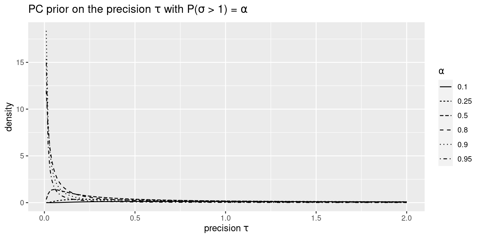
Figure 5.1: PC priors for the precision $\tau$.

5.5 Sensitivity analysis with R-INLA

Given the speed at which models are fitted with INLA it is possible to conduct a sensitivity analysis on the priors in the model. This is important because the choice of the priors can have an important impact on the posterior distributions of the model parameters.

We will go back to the dataset described in Section 4.4 on the performance of children at school. The dataset can be loaded as follows:

csize_data <- read.csv (file = "data/class_size_data.txt", header = FALSE,
  sep = "", dec = ".")

#Set names
names(csize_data) <- c("clsnr", "pupil", "nlitpre", "nmatpre", "nlitpost",
  "nmatpost", "csize")

#Set NA's
csize_data [csize_data < -1e+29 ] <- NA

#Set class size levels
csize_data$csize <- as.factor(csize_data$csize)
levels(csize_data$csize) <- c("<=19", "20-24", "25-29", ">=30")

In the sensitivity analysis we will compare the default prior with INLA and the priors defined in the previous section. All these priors will be put together in a list so that different models are fit by looping over this list.

prior.list = list(
  default = list(prec = list(prior = "loggamma", param = c(1, 0.00005))),
  half.normal = list(prec = list(prior = HN.prior)),
  half.cauchy = list(prec = list(prior = HC.prior)),
  h.t = list(prec = list(prior = HT.prior)),
  uniform = list(prec = list(prior = UN.prior)),
  pc.prec = list(prec = list(prior = "pc.prec", param = c(5, 0.01)))
)

Before proceeding to fit the models with INLA, the rows with missing values in the first 4 columns of the dataset are removed. INLA will remove them anyway, but we prefer to make this step explicit and create a new dataset csize_data2 for model fitting:

#Remove rows with NA's
csize_data2 <- na.omit(csize_data[, -5])

Model fitting is done with the lapply() function so that each prior in list prior.list is used in turn:

csize.models <- lapply(prior.list, function(tau.prior) {
  inla(nmatpost ~ 1 + nmatpre + nlitpre + csize +
      f(clsnr, model = "iid", hyper = tau.prior), data = csize_data2,
    control.family = list(hyper = tau.prior))
})

The posterior marginals of the error precision $\tau_e$ and the iid random effect $\tau_u$ for the different priors used have been plotted in Figure 5.2. In this particular case no differences can be appreciated.

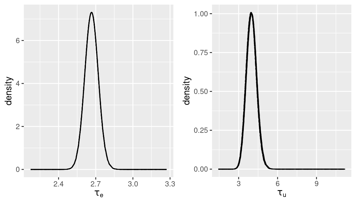
Figure 5.2: Sensitivity analysis on the priors of the precisions of the model.

5.6 Scaling effects and priors

As mentioned in Chapter 3, latent effects in INLA can be scaled in different ways and this may require a different prior setting. Scaling is particularly important for intrinsic models, such as the random walk latent effects or some of the spatial models described in Section 7.2.2. Sørbye (2013) and Sørbye and Rue (2014) provide more details on how the scaling is done in INLA.

Briefly, scaling a model means that the generalized variance of the latent effect is one (see Sørbye 2013 for details). This scaling will take the values of the scale hyperparameter to a different range, which implies that different priors should be used for scaled and unscaled models. In addition, this also means that precision estimates are comparable between different models and that estimates are less affected by re-scaling covariates in the linear predictor. Furthermore, re-scaling makes the precision invariant to changes in the shape and size of the latent effect.

Scaling is done through arguments scale and scale.model in the definition of the latent effects via the f() function. See Table 5.5.

Table 5.5: Arguments that can be passed to the `f()` function for model scaling.
Argument	Default	Description
`scale`	`NULL`	A scaling vector.
`scale.model`	`NULL`	Scale model (if `TRUE`).

Scaling latent effects means that the generalized variance is taken to be equal to one. As a result, precision parameters in the latent effects are comparable and they can take the same prior distribution.

In order to show how scaling affects model fitting we will use the lidar dataset described in detail in Chapter 9. We will consider the same non-parametric models using rw1 and rw2 latent effect with and without re-scaling the models:

library("SemiPar")
data(lidar)

#Data for prediction
xx <- seq(390, 720, by = 5)
# Add data for prediction
new.data <- cbind(range = xx, logratio = NA)
new.data <- rbind(lidar, new.data)

# Set prior on precision
prec.prior <- list(prec = list(param = c(0.001, 0.001)))

#RW1 latent effect
m.rw1 <- inla(logratio ~ 1 + f(range, model = "rw1", constr = FALSE,
    hyper = prec.prior),
  data = new.data, control.predictor = list(compute = TRUE))
#RW1 scaled latent effect
m.rw1.sc <- inla(logratio ~ 1 + f(range, model = "rw1", constr = FALSE,
    scale.model = TRUE, hyper = prec.prior),
  data = new.data, control.predictor = list(compute = TRUE))

#RW2 latent effect
m.rw2 <- inla(logratio ~ 1 + f(range, model = "rw2", constr = FALSE,
    hyper = prec.prior),
  data = new.data, control.predictor = list(compute = TRUE))
#RW2 scaled latent effect
m.rw2.sc <- inla(logratio ~ 1 + f(range, model = "rw2", constr = FALSE,
    scale.model = TRUE,  hyper = prec.prior),
  data = new.data, control.predictor = list(compute = TRUE))

Note that in the previous code, the priors for the precision parameters of the scaled models is a Gamma with parameters $0.001$ and $0.001$, instead of the default values of $1$ and $0.00005$ to provide a vague prior (as discussed in Chapter 3). This is required because the precision parameters in the scaled models are in a completely different scale and the default prior does not make much sense now as it provides an extremely large prior variance of the precision parameter. Also, by setting the same prior for all models we can appreciate the effects of scaling a model better.

Table 5.7 shows the different estimates of the precisions of the rw1 and rw2 latent effects. As can be seen, the precision parameters of the scaled models are comparable, while the corresponding parameters for the un-scaled models are in completely different ranges (Sørbye 2013). This scaling effect is similar to the one observed in the examples on scaling random effects in Chapter 3.

Table 5.6: Table: Table 5.7: Summary of the posterior distribution of the precision hyperparameters for different scaled and un-scaled intrinsic latent effects.
Model	Scaled	Mean	St. dev.	0.025 quant.	0.975 quant.
`rw1`	No	52.85	1.11	50.73	55.09
`rw1`	Yes	47.39	1.50	43.96	49.60
`rw2`	No	122.82	1.23	120.50	125.39
`rw2`	Yes	73.78	0.22	73.33	74.24

Table: (#tab:lidarscaling)Summary of the posterior distribution of the precision hyperparameters for different scaled and un-scaled intrinsic latent effects.

Regarding the fitted model, Figure 5.3 shows the different models fit to the data. Both scaled and unscaled models produce very similar estimates. However, scaled models seem to produce smoother curves, which may also be an effect of the priors used.

5.7 Final remarks

Prior definition in INLA is flexible enough to consider many different types of approaches which in turn allow us to fit wider types of models. In particular, PC priors are particularly well suited for the INLA methodology and the modular model definition of additive models. INLA also has the capability of re-scaling intrinsic latent effects so that the estimates of the precision do not depend on the shape and size of the latent effect and re-scaled covariates in the model.

Other priors may be implemented in INLA in a number of ways. For example, when new latent effects are implemented (as explained in Section 11) priors need to be set explicitly using appropriate R functions. This means that priors not implemented in INLA but available in R can be used. This includes, for example, multivariate priors or priors that do not fit within the INLA framework (Gómez-Rubio and HRue 2018).

Multivariate priors could, in principle, be used with INLA and a few latent effects have them implemented. However, most of the priors available in INLA are univariate. Multivariate priors could be included in the latent effects by implementing them using the methods described in Chapter 11. This is so because the prior of the hyperparameters needs to be explicitly computed using R code and, hence, this will allow us to include multivariate priors. Palmí-Perales, Gómez-Rubio, and Martínez-Beneito (2019) use the rgeneric feature described in Chapter 11 to implement new latent effects for multivariate data and some of the models require multivariate priors. Those examples can be used as a template to implement latent effects that use multivariate priors.

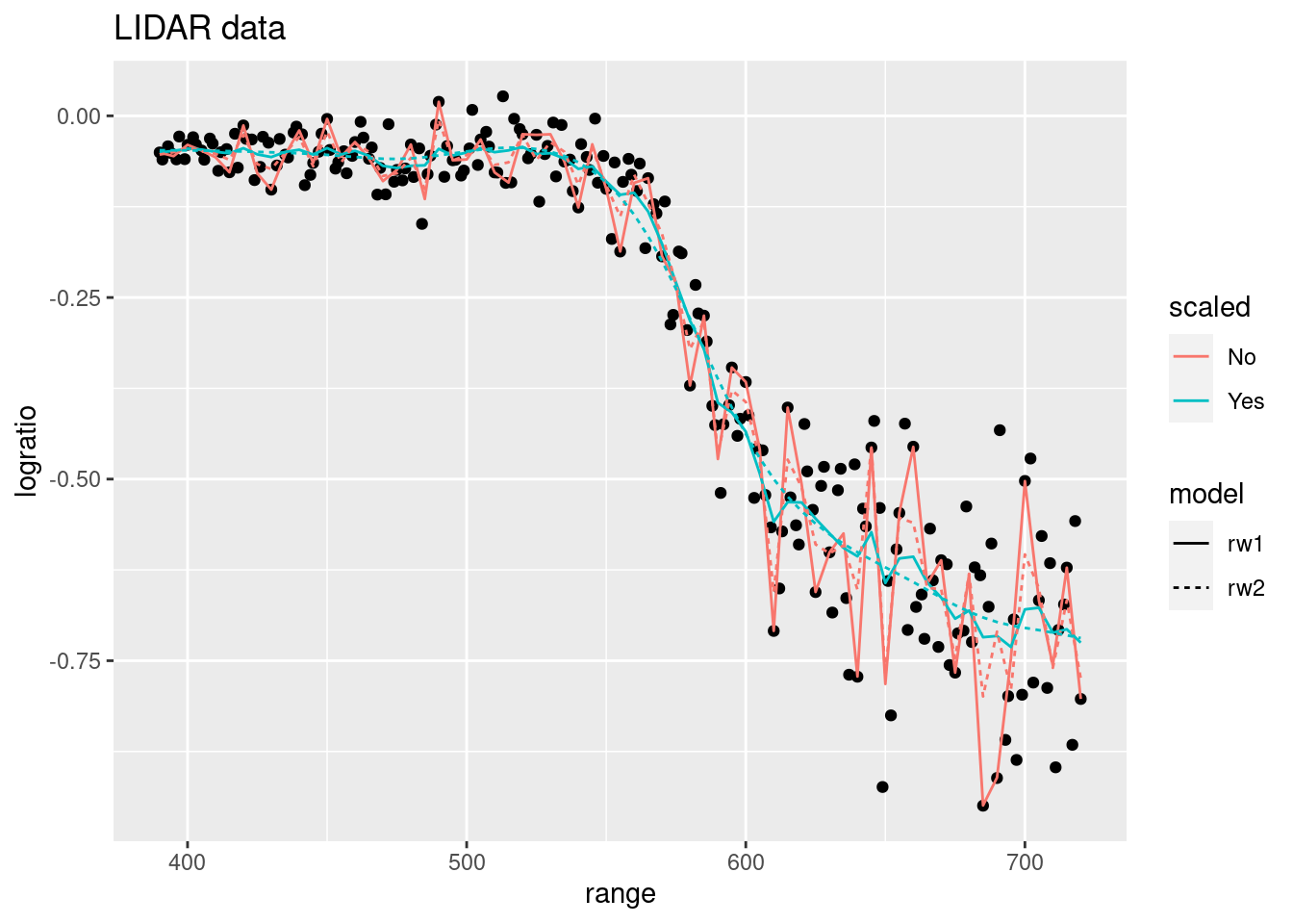
Figure 5.3: Fitted values of the lidar dataset using scaled and unscaled latent effects.

References

Gelman, A. 2006. “Prior Distributions for Variance Parameters in Hierarchical Models.” Bayesian Analysis 1 (3): 515–34.

Gómez-Rubio, Virgilio, and HRue. 2018. “Markov Chain Monte Carlo with the Integrated Nested Laplace Approximation.” Statistics and Computing 28 (5): 1033–51.

Gómez-Rubio, Virgilio, Francisco Palmí-Perales, Gonzalo López-Abente, Rebeca Ramis-Prieto, and Pablo Fernández-Navarro. 2019. “Bayesian Joint Spatio-Temporal Analysis of Multiple Diseases.” SORT 43 (1): 51–74.

Palmí-Perales, Francisco, Virgilio Gómez-Rubio, and Miguel A. Martínez-Beneito. 2019. “Bayesian Multivariate Spatial Models for Lattice Data with INLA.” arXiv E-Prints, September, arXiv:1909.10804. http://arxiv.org/abs/1909.10804.

Simpson, D. P., H. Rue, A. Riebler, T. G. Martins, and S. H. Sørbye. 2017. “Penalising Model Component Complexity: A Principled, Practical Approach to Constructing Priors.” Statistical Science 32 (1): 1–28.

Sørbye, Sigrunn Holbek. 2013. Tutorial: Scaling Igmrf-Models in R-Inla.

Sørbye, Sigrunn Holbek, and Håvard Rue. 2014. “Scaling Intrinsic Gaussian Markov Random Field Priors in Spatial Modelling.” Spatial Statistics 8: 39–51. https://doi.org/https://doi.org/10.1016/j.spasta.2013.06.004.

Ugarte, María Dolores, Aritz Adin, and Tomás Goicoa. 2016. “Two-Level Spatially Structured Models in Spatio-Temporal Disease Mapping.” Statistical Methods in Medical Research 25 (4): 1080–1100. https://doi.org/10.1177/0962280216660423.

Wang, Xiaofeng, Yu Yue Ryan, and Julian J. Faraway. 2018. Bayesian Regression Modeling with Inla. Boca Raton, FL: Chapman & Hall/CRC.

Parameter	Range	Internal	\(f(\theta)\)	\(\|\partial f(\theta)/ \partial\theta\|\)
Precision \(\tau\)	\((0, \infty)\)	\(\theta = \log(\tau)\)	\(\tau = \exp(\theta)\)	\(\exp(\theta)\)
Variance \(\sigma^2\)	\((0, \infty)\)	\(\theta = -\log(\sigma^2)\)	\(\sigma^2 = \exp(-\theta)\)	\(\exp(-\theta)\)
St. dev. \(\sigma\)	\((0, \infty)\)	\(\theta = -2\log(\sigma)\)	\(\sigma = \exp(-\theta/2)\)	\(\exp(-\theta/2) / 2\)
Correlation \(\rho\)	\((-1, 1)\)	\(\theta = \log(\frac{1 + \rho}{1 - \rho})\)	\(\rho = 2 \frac{\exp(\theta)}{1 + \exp(\theta)} -1\)	\(2\exp(\theta) / (1 +\exp(\theta))^2\)
Coefficient \(\beta\)	\((0, 1)\)	\(\theta = \log(\frac{\beta}{1 - \beta})\)	\(\beta = \frac{\exp(\theta)}{1 + \exp(\theta)}\)	\(\exp(\theta) / (1 +\exp(\theta))^2\)

Prior	Parameter	Hyperparameters	Base model	Definition
`pc.prec`	Precision \(\tau = \sigma^{-2}\)	\((\sigma_0, \alpha)\)	\(\sigma = 0\)	\(P(\sigma > \sigma_0) = \alpha\)
`pc.dof`	Degrees of freedom \(\nu\)	\((u, \alpha)\)	\(\nu = \infty\)	\(P(\nu < u) = \alpha\)
`pc.cor0`	Correlation \(\rho\)	\((\rho_0, \alpha)\)	\(\rho = 0\)	\(P(\|\rho\| > \rho_0) = \alpha\)
`pc.cor1`	Correlation \(\rho\)	\((\rho_0, \alpha)\)	\(\rho = 1\)	\(P(\rho > \rho_0) = \alpha\)