Chapter 11 Implementing New Latent Models

11.1 Introduction

In previous chapters we have covered several latent effects implemented in the INLA package. These include a number of important and popular latent effects that are widely used. However, it may be the case that an unimplemented latent effect is required in our model. Given that most of the latent effects are implemented in a mix of C and R code, it is difficult to add new latent effects to the INLA package directly.

The INLA methodology can handle many more latent effects than those included in the INLA package. For this reason, we will describe now how to add new latent effects. In particular, the spatial autoregressive model described in Section 11.2 will be considered. The implementation of this new latent effect will be done considering three different approaches. In Section 11.3 we will cover the rgeneric latent effect that allows new latent effects implemented in R code. In Section 11.4 we describe a novel approach to fit unimplemented latent effects by means of Bayesian model averaging (BMA, Hoeting et al. 1999; Gómez-Rubio, Bivand, and Rue 2019). Finally, in Section 11.5 we describe how to combine INLA and MCMC (Gómez-Rubio and HRue 2018) to increase the number of models that can be fitted using INLA.

11.2 Spatial latent effects

As a case study, we will show how to implement a spatial model. In particular, we will consider the conditionally autoregressive (CAR) specification (Banerjee, Carlin, and Gelfand 2014). Now, the latent effects have a Gaussian distribution with zero mean and precision matrix

\[ \Sigma = \tau (I - \rho W) \]

Here, \(\tau\) is a precision hyperparameter, \(\rho\) is a spatial autocorrelation parameter and \(W\) is a binary adjacency matrix. \(\Sigma\) is a very sparse matrix given that both \(I\) and \(W\) are very sparse matrices.

Note that matrix \(W\) must be provided. This can be easily obtained by loading some spatial data from R. For example, we will consider the North Carolina SIDS dataset that was analyzed in Section 2.3.2. However, a spatial analysis will be considered now. First of all, a shapefile with the data will be loaded and the expected number of cases, standardized mortality ratios and proportion of non-white births per county in the period will be computed:

library("spdep")
library("rgdal")

SIDS <- readOGR(system.file("shapes/sids.shp", package="spData")[1])
proj4string(SIDS) <- CRS("+proj=longlat +ellps=clrk66")

#Expected cases
SIDS$EXP74 <- SIDS$BIR74 * sum(SIDS$SID74) / sum(SIDS$BIR74)
#Standardised Mortality Ratio
SIDS$SMR74 <- SIDS$SID74 / SIDS$EXP74
#Proportion of non-white births
SIDS$PNWB74 <- SIDS$NWBIR74 / SIDS$BIR74

Figure 11.1 shows the standardized mortality ratio (i.e., observed divided by expected cases) in each county in North Carolina.

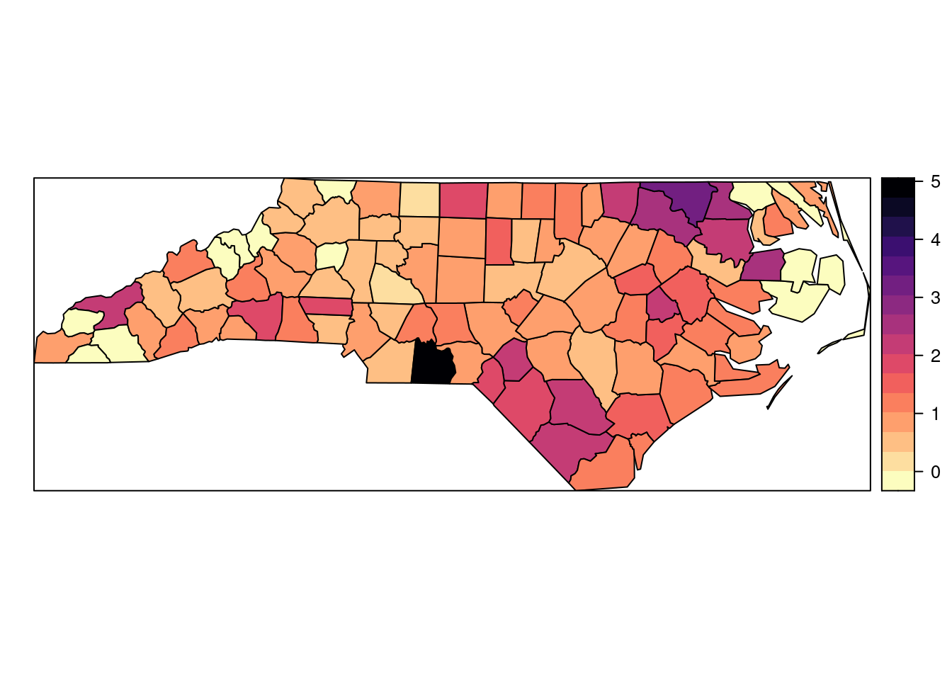
Figure 11.1: Standardised mortality ratio of the North Carolina SIDS dataset for the period 1971-1974.

Next, a binary adjacency matrix needs to be computed using function poly2nb:

#Adjacency matrix
adj <- poly2nb(SIDS)
W <- as(nb2mat(adj, style = "B"), "sparseMatrix")

This model is well defined when \(\rho\) is in the range \((1/\lambda_{min}, 1/\lambda_{max})\), where \(\lambda_{min}\) and \(\lambda_{max}\) are the minimum and maximum eigenvalues of \(W\), respectively. Hence, we will compute this first:

e.values <- eigen(W)$values
rho.min <- min(e.values)
rho.max <- max(e.values)

In order to have the spatial autocorrelation parameter constrained to be lower than 1 (see, for example, Haining 2003 for details), the adjacency matrix will be re-scaled by dividing by \(\lambda_{max}\):

#Re-scale adjacency matrix
W <- W / rho.max

Usually, the range of the spatial autocorrelation parameter will be considered to be \((0, 1)\), so that it can be interpreted similarly as a correlation parameter.

11.3 R implementation with rgeneric

The rgeneric latent effect is a mechanism implemented in the INLA package to allow users to implement latent effects in R. This is possible because R can be embedded into other front-end programs in a way that allows R code to be run from C (R Core Team 2019b). A detailed description of this feature can be accessed by typing inla.doc('rgeneric').

The definition of a new latent effect requires the definition of the latent effect as a GMRF. This means that the mean and precision matrix of the GRMF need to be defined, as well as the hyperparameters \(\bm\theta\) involved and their prior distributions.

Specifying the latent effect as a GMRF also requires a binary representation of the precision matrix to exploit conditional independence properties. i.e., a ‘graph’. This is simply a matrix of the same dimension as the precision matrix with entries equal to zero where the precision matrix is zero and 1 otherwise. When passing this graph matrix to define an rgeneric latent effect, the precision matrix can be used as well regardless of whether it is binary or not.

To sum up, in order to define a new latent effect, the following need to be defined using several R functions:

• The mean of the latent effects \(\mu(\theta)\).

• The precision of the latent effects \(Q(\theta)\).

• A ‘graph’, with a binary representation of the precision matrix.

• The initial values of \(\theta\).

• A log-normalizing constant.

• The log-prior of \(\theta\).

Before starting coding all this, it is important to provide an internal representation of the hyperparameters that make numerical optimization easier. As a rule, it is good to have a reparameterization of the parameters so that the internal parameters are not bounded as this will simplify computations. In particular, we will use \(\theta_1 = \log(\tau)\) and \(\theta_2 = logit(\rho)\).

INLA will internally work with parameters \((\theta_1, \theta_2)\). For this reason, we will need first to define the following function to convert the hyperparameters from the internal scale to the model scale, i.e, to obtain parameters \((\tau, \rho)\) from \((\theta_1, \theta_2)\):

\[ \tau = \exp(\theta_1) \]

\[ \rho = \frac{1}{1 + \exp(-\theta_2)} \]

A variable theta is defined by INLA in the code to store \(\theta = (\theta_1, \theta_2)\). So, the following function interpret.theta will take the parameters in the internal scale and return the precision and spatial autocorrelation parameters:

interpret.theta <- function() {
  return(
    list(prec = exp(theta[1L]),
    rho = 1 / (1 + exp(-theta[2L])))
  )
}

Next, we will define the ‘graph’, which essentially defines what entries of the precision matrix are non-zero. Note that this is a matrix of the same size as the precision matrix and that \(W\) must be passed as a sparse matrix (as defined in package Matrix) and the returned matrix must be sparse too.

graph <- function(){
  require(Matrix)

  return(Diagonal(nrow(W), x = 1) + W)
}

The precision matrix is defined in a similar way:

Q <- function() {
  require(Matrix)

  param <- interpret.theta()

  return(param$prec * (Diagonal(nrow(W), x = 1) - param$rho * W) )
}

The mean can be defined very easily now because it is zero:

mu = function()
{
  return(numeric(0))
}

The logarithm of the normalizing constant in this case is the typical normalizing constant of a multivariate Gaussian distribution:

log.norm.const <- function() {
  param <- interpret.theta()
  n <- nrow(W)

  Q <- param$prec * (Diagonal(nrow(W), x = 1) - param$rho * W)

  res <- n * (-0.5 * log(2 * pi)) +
    0.5 * Matrix::determinant(Q, logarithm = TRUE)

  return(res)
}

Note that INLA will compute this normalizing constant if numeric(0) is returned, so this can be omitted.

The log-prior must be specified in another function. For precision \(\tau\), we will be using a gamma distribution with parameters \(1\) and \(0.00005\), and for \(\rho\) a uniform distribution on \((0,1)\):

log.prior <- function() {
  param = interpret.theta()

  res <- dgamma(param$prec, 1, 5e-05, log = TRUE) + log(param$prec) +
      log(1) + log(param$rho) + log(1 - param$rho)

  return(res)
}

Note that the extra terms that appear in the definition of the log-density of the prior are due to the change of variable involved. INLA works with \((\theta_1,\theta_2)\) internally, but the prior is set on \((\tau, \rho)\). See Chapter 5 for details on how to set the prior properly.

Finally, a function to set the initial values of the parameters in the internal scale must be provided:

initial <- function() {
  return(rep(0, 0))
}

This implies that the initial values of \(\tau\) and \(\rho\) are \(1\) and \(0.5\), respectively.

A quit() function is called when all computations are finished before exiting the C code. In this case, we will simply return nothing.

quit <- function() {
  return(invisible())
}

The actual definition of the latent effect is done via function inla.rgeneric.define. This function takes as first argument the functions defined before and some extra arguments needed to evaluate the different functions:

'inla.rgeneric.CAR.model' <- function(
  cmd = c("graph", "Q", "mu", "initial", "log.norm.const",
    "log.prior", "quit"),
  theta = NULL) {

  #Internal function
  interpret.theta <- function() {
    return(
      list(prec = exp(theta[1L]),
      rho = 1 / (1 + exp(-theta[2L])))
    )
  }

  graph <- function(){
    require(Matrix)

    return(Diagonal(nrow(W), x = 1) + W)
  }

  Q <- function() {
    require(Matrix)

    param <- interpret.theta()

    return(param$prec * (Diagonal(nrow(W), x = 1) - param$rho * W) )
  }

  mu <- function()
  {
    return(numeric(0))
  }

  log.norm.const <- function() {
    return(numeric(0))

  }

  log.prior <- function() {
    param = interpret.theta()

    res <- dgamma(param$prec, 1, 5e-05, log = TRUE) + log(param$prec) +
      log(1) + log(param$rho) + log(1 - param$rho) 

    return(res)
  }

  initial <- function() {
    return(c(0, 0))
  }

  quit <- function() {
    return(invisible())
  }

  res <- do.call(match.arg(cmd), args = list())
  return(res)
}

Then, the model is defined to be used by INLA using function inla.rgeneric.define as follows:

library("INLA")

CAR.model <- inla.rgeneric.define(inla.rgeneric.CAR.model, W = W)

Note that inla.rgeneric.define() takes as first argument the function that defines the latent effect followed by a sequence of named arguments with variables that are required in the computation of the latent effect. In this case, matrix W is the adjacency matrix required by the CAR latent effect but more arguments could follow when needed.

The model can now be fitted as follows:

SIDS$idx <- 1:nrow(SIDS)

f.car <- SID74 ~ 1 + f(idx, model = CAR.model)

m.car <- inla(f.car, data = as.data.frame(SIDS), family = "poisson",
  E = SIDS$EXP74)#, control.inla = list(tolerance = 1e-20, h = 1e-4))

A summary of the model can be obtained as usual:

summary(m.car)

## 
## Call:
##    c("inla(formula = f.car, family = \"poisson\", data = 
##    as.data.frame(SIDS), ", " E = SIDS$EXP74)") 
## Time used:
##     Pre = 0.405, Running = 2.59, Post = 0.0271, Total = 3.02 
## Fixed effects:
##              mean    sd 0.025quant 0.5quant 0.975quant  mode kld
## (Intercept) 0.034 0.109     -0.172     0.03       0.26 0.022   0
## 
## Random effects:
##   Name     Model
##     idx RGeneric2
## 
## Model hyperparameters:
##                mean    sd 0.025quant 0.5quant 0.975quant mode
## Theta1 for idx 2.20 0.331      1.562     2.19       2.86 2.16
## Theta2 for idx 2.30 1.163      0.108     2.27       4.67 2.15
## 
## Expected number of effective parameters(stdev): 36.73(6.24)
## Number of equivalent replicates : 2.72 
## 
## Marginal log-Likelihood:  -241.04

The marginals of the hyperparameters are in the internal scale and they need to be transformed:

marg.prec <- inla.tmarginal(exp, m.car$marginals.hyperpar[[1]])
marg.rho <- inla.tmarginal(function(x) { 1/(1 + exp(-x))},
  m.car$marginals.hyperpar[[2]])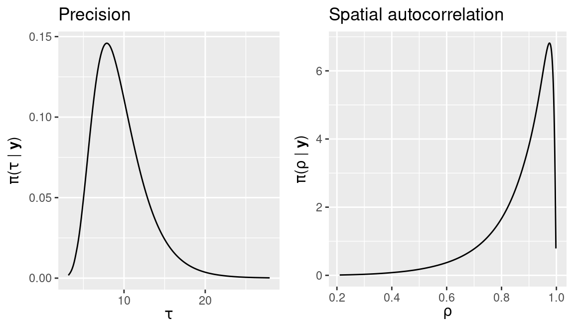

Figure 11.2: Posterior marginals of parameters \(\tau\) and \(\rho\) of the proper CAR latent model for the SIDS dataset.

Figure 11.2 shows the posterior marginals of \(\tau\) and \(\rho\). These show a strong spatial autocorrelation. Finally, summary statistics on these parameters can be obtained with inla.zmarginal (see Section 2.6):

inla.zmarginal(marg.prec, FALSE)

## Mean            9.49098 
## Stdev           3.25664 
## Quantile  0.025 4.78851 
## Quantile  0.25  7.16016 
## Quantile  0.5   8.91091 
## Quantile  0.75  11.1926 
## Quantile  0.975 17.4427

inla.zmarginal(marg.rho, FALSE)

## Mean            0.867327 
## Stdev           0.122387 
## Quantile  0.025 0.52924 
## Quantile  0.25  0.818303 
## Quantile  0.5   0.906084 
## Quantile  0.75  0.955611 
## Quantile  0.975 0.990365

Posterior means of the random effects have been plotted in a map in Figure 11.3. It shows the underlying spatial pattern of the risk from SIDS. It should be mentioned that the spatial pattern of the proportion of non-white births is very similar to the one shown in Figure 11.3 and that is why when this covariate is included in the model (as discussed in Section 2.3.2) it accounts for most of the overdispersion in the data and random effects are not required any more.

SIDS$CAR <- m.car$summary.random$idx[, "mean"]
spplot(SIDS, "CAR",  col.regions = rev(inferno(16)))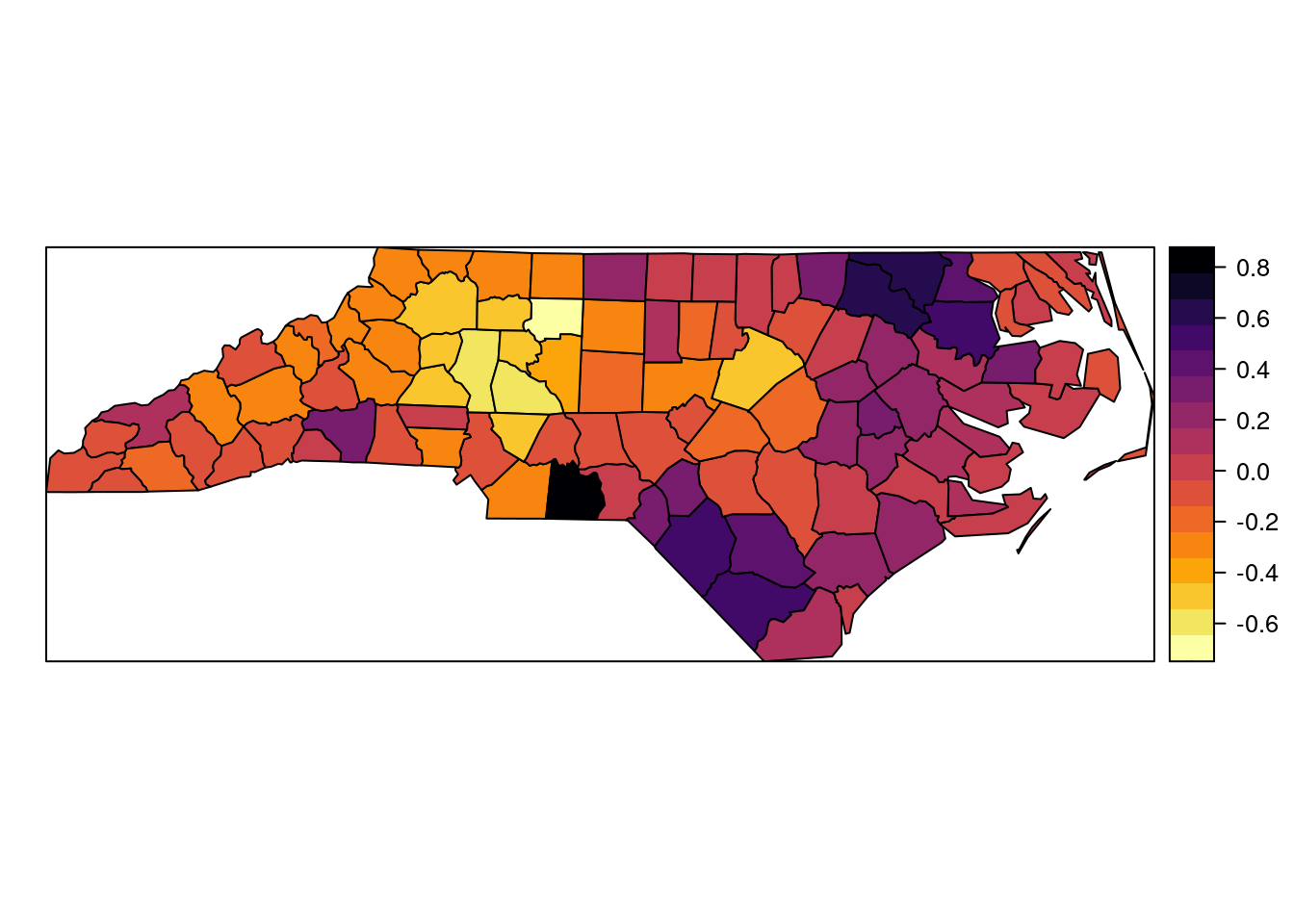

Figure 11.3: Posterior means of the CAR random effects.

11.4 Bayesian model averaging

Bivand, Gómez-Rubio, and HRue (2014) describe a novel approach to fit new models with INLA. Their approach is based on conditioning on one of the hyperparameters in the model and fit conditional models on several values of this parameter. Then, all models are combined using Bayesian model averaging (BMA, Hoeting et al. 1999) to obtain the posterior marginals of all the parameters in the model. Bivand, Gómez-Rubio, and HRue (2014) use this approach to fit a number of spatial econometrics models, which are available in package INLABMA (Bivand, Gómez-Rubio, and Rue 2015). Recently, Gómez-Rubio, Bivand, and Rue (2019) have extended the work in Bivand, Gómez-Rubio, and HRue (2014) to consider a wider family of spatial econometrics models.

In the case of the CAR specification, it is worth noting that, given \(\rho\), the resulting model can be implemented using a generic0 latent effect because the structure of the precision matrix is known and only hyperparameter \(\tau\) needs to be estimated. By giving values to \(\rho\) in a bounded interval the posterior marginal of \(\rho\) can be computed as well by Bayesian model averaging.

First of all, we will create a function that will take a value of \(\rho\) and the adjacency matrix \(W\) and fit the CAR model conditional on \(\rho\):

car.inla <- function(formula, d, rho, W, ...) {

  #Create structure of precision matrix I - rho * W
  IrhoW <- Matrix::Diagonal(nrow(W), x = 1) - rho * W

  #Add CAR index
  d$CARidx <- 1:nrow(d)

  formula <- update(formula, . ~ . + f(CARidx, model = "generic0", 
            Cmatrix = IrhoW))
  res <- inla(formula, data = d, ..., control.compute = list(mlik = TRUE),
    control.inla = list(tolerance = 1e-20, h = 1e-4))

  #Update mlik
  logdet <- determinant(IrhoW)$modulus
  res$mlik <- res$mlik + logdet / 2

  return(res)
}

Note that the log-marginal likelihood needs to be corrected to account for the structure of the precision matrix and this is why term logdet / 2 is added to the value of the marginal likelihood. By default, INLA will not compute it in this case because it assumes that the structure of the precision matrix is known. Hence, its determinant is constant and does not need to be computed and only the precision hyperparameter \(\tau\) is accounted for when computing the marginal likelihood. Furthermore, control.inla has been used to set the values of tolerance and h to obtain accurate estimates of the marginal likelihood.

Next, a regular grid of points in the domain of \(\rho\) where to evaluate the model is required. In this case, the domain is the interval \((0, 1)\) and the grid points will be denoted by \(\{\rho^{(i)}\}_{i=1}^N\), where \(N\) is the number of points. For this particular case, as we already know that the region of high probability of the posterior marginal of \(\rho\) is very close to one, the grid will be made of 100 points from \(0.5\) to \(1\):

rho.val <- seq(0.5, 1, length.out = 100)

It should be noted that values very close to 1 may cause computational problems because the precision matrix becomes almost singular.

Next, we evaluate the model at all these points. Although this involves fitting a large number of models, these can be fitted in parallel using function mclapply. In the next lines, the parallel library will be loaded and set up to use 4 cores before fitting the conditional models:

library("parallel")
options(mc.cores = 4)

Model fitting will be in parallel and we set each parallel INLA process to use a single core (by setting num.threads to 1):

car.models <- mclapply (rho.val, function(rho) {
    car.inla(SID74 ~ 1, as.data.frame(SIDS), rho, W, 
      family = "poisson", E = SIDS$EXP74, 
      num.threads = 1)
})

When INLA is used to fit several models in parallel on the same machine it is convenient to set the number of threads used by each INLA process to a value that ensures that no more cores than available are used. For example, in the previous example, the mclapply loop will be using 4 cores (as set in mc.cores), which means that 4 INLA processes will be run. Each one of these processes will be using 1 core at a time (as set in num.threads), so that altogether 4 cores are used. Similarly, if the total number of cores is 8, then num.threads could be set to 2 so that each INLA process takes 2 cores and the total number of cores used is 8.

Then, we have a number of conditional models on \(\rho\) that we can combine to obtain the desired model. These models will be combined using Bayesian model averaging, which is the appropriate way of combining models.

Note that, given any particular value of \(\rho\), the fitted conditional model with INLA will provide the conditional marginals of the parameters, \(\pi(\cdot \mid \rho)\), and the conditional marginal likelihood \(\pi(\mathbf{y} \mid \rho)\). The posterior marginal of \(\rho\) can be obtained as:

\[ \pi(\rho \mid \mathbf{y}) = \frac{\pi(\mathbf{y} \mid \rho)\pi(\rho)}{\pi(\mathbf{y})} \propto \pi(\mathbf{y} \mid \rho)\pi(\rho) \]

This can be computed from the previous output because \(\pi(\mathbf{y} \mid\rho)\) is the conditional marginal likelihood for a conditional model on \(\rho\) and \(\pi(\rho)\) is the value of the prior on \(\rho\) (which is known and equal to 1 in this case). \(\pi(\mathbf{y})\) is a constant that can be ignored as the posterior marginal can be re-scaled to integrate 1.

In practice, we will estimate the value of the posterior marginals at the points of the grid, fit a smooth function and then re-scale the resulting function to integrate 1, so that we have a proper density function. Here, this is done by function INLABMA but function inla.merge() could have also been used (as shown in the next section):

library("INLABMA")
car.bma <- INLABMA(car.models, rho.val, log(1))

The posterior marginal of \(\rho\) estimated with this method can be seen in Figure 11.5, which also includes two other estimates using different approaches explained below.

If required, the log-marginal likelihoods (conditional on \(\rho\)) from the fit models can be easily obtained with:

#Obtain log-marginal likelihoods
mliks <- unlist(lapply(car.models, function(X){X$mlik[1, 1]}))

The posterior marginals for the remainder of latent effects and hyperparameters in the model can be computed by integrating \(\rho\) out. For example, for a hyperparameter \(\theta_t\) (and similarly for any latent effect) this would mean:

\[ \pi(\theta_t \mid \mathbf{y}) = \int \pi(\theta_t , \rho \mid \mathbf{y}) d\rho = \int \pi(\theta_t \mid \mathbf{y}, \rho) \pi(\rho \mid \mathbf{y}) d\rho \]

Taking a set of values of \(\rho\) in a grid \(\{\rho^{(i)}\}_{i=1}^N\), this can be approximated by the following expression (Bivand, Gómez-Rubio, and HRue 2014):

\[ \pi(\theta_t \mid \mathbf{y}) \simeq \sum_{i=1}^N \pi(\theta_t \mid \mathbf{y}, \rho^{(i)}) w_i \]

with weights \(w_i\) equal to

\[ w_i = \frac{\pi(\mathbf{y} \mid \rho^{(i)}) \pi(\rho^{(i)}) } {\sum_{i=1}^N \pi(\mathbf{y}\mid \rho^{(i)}) \pi(\rho^{(i)})} \]

Note the approximation to \(\pi(\theta_t \mid \mathbf{y})\) can be regarded as Bayesian model averaging (Hoeting et al. 1999), as it is a weighted sum of conditional posterior marginals from different models.

Function INLAMH() computes this model average to obtain the marginals of the other hyperparameters and latent effects in the model. See Bivand, Gómez-Rubio, and Rue (2015) for details. The summaries of the coefficients of the fixed effects and the hyperparameters can be obtained as follows:

# Fixed effects
car.bma$summary.fixed

##               mean     sd 0.025quant 0.5quant 0.975quant    mode       kld
## (Intercept) 0.0336 0.1011    -0.1717  0.03573      0.227 0.03983 6.082e-12

It is worth mentioning that function inla.merge() can also compute the average of the posterior marginals from different models (see next section). In this case, each model has a different weight \(w_i\) that must be passed to the inla.merge() function in order to obtain the right model.

11.5 INLA within MCMC

Finally, the third approach that will be discussed to use INLA to fit models with unimplemented latent effects is based on Gómez-Rubio and HRue (2018). They point out that the approach in Bivand, Gómez-Rubio, and HRue (2014) is useful for a very small number of hyperparameters with bounded support. However, when the hyperparameters do not have a bounded support or there are many of them, simple numerical approximations will be difficult to implement.

For this reason, Gómez-Rubio and HRue (2018) propose the use of INLA within the Metropolis-Hastings algorithm so that the hyperparameter space is conveniently explored. The main idea is to split the set of hyperparameters into two groups, so that conditional on one of the subsets the resulting model can be easily fitted with INLA. This is essentially what we have done in Section 11.4 when fitting models conditional on \(\rho\).

Function INLAMH, in package INLABMA, implements the INLA within Metropolis-Hastings algorithm. It requires a function to fit the model conditional on some of the hyperparameters, two functions (that implement the proposal distribution) to sample new values of the hyperparameters and compute its density, and the prior of the hyperparameters.

Similarly as in Section 11.4, the models fitted with INLA will be conditional on \(\rho\), and the marginal distribution of \(\rho\) will be obtained from the samples from the Metropolis-Hastings algorithm.

The function to fit a model conditional on \(\rho\) is the following:

fit.inla <- function(d, x){
  #Rho
  rho <- x

  res <- car.inla(SID74 ~ 1, d, rho, W,
    family = "poisson", E = d$EXP74)

  return(list(model.sim = res, mlik = res$mlik[1, 1]))
}

This function returns a list with the fit model (model.sim) and the estimate of the marginal likelihood (mlik).

The function used to propose new values of \(\rho\), in the logit-scale, will be a Gaussian centered at the current value with a small precision. For this, function rlogitnorm from package logitnorm(Wutzler 2018) will be used. By using this function we avoid dealing with changes in the scale of the parameters (see Chapter 5 for details).

library("logitnorm")
#Sample values of rho
rq.rho <- function(x, sigma = 0.15) {
  rlogitnorm(1, mu = logit(x), sigma = sigma)
}

#Log-density of proposal distribution
dq.rho <- function(x, y, sigma = 0.15, log = TRUE) {
  dlogitnorm(y, mu = logit(x), sigma = sigma, log = log)
}

Here, x represents the current value of \(\rho\), y the proposed value and sigma is the standard deviation of the proposal distribution. Note also that the density is returned in the log-scale.

Finally, we need to set the prior on \(\rho\):

#Log-density of prior
prior.rho <- function(rho, log = TRUE) {
  return(dunif(rho, log = log))
}

Once all the required functions have been defined, the INLAMH function can be called to run the INLA with MCMC algorithm. In the next lines, the starting point for \(\rho\) is set to 0.95:

inlamh.res <- INLAMH(as.data.frame(SIDS), fit.inla, 0.95, rq.rho, dq.rho,
  prior.rho,
  n.sim = 100, n.burnin = 100, n.thin = 5, verbose = TRUE)

The resulting object inlamh.res is a list with three elements:

• acc.sim, indicates whether the proposed value of \(\rho\) was accepted or not, and it is useful to compute the acceptance rate.

• model.sim is a list with the conditional models fitted with INLA.

• b.sim is a list with the values of \(\rho\). In this case, each element in the list is a vector of length one, but this can take many other forms.

A simple way to put all the samples from \(\rho\) together is the following:

rho.sim <- unlist(inlamh.res$b.sim)

Figure 11.4 displays the samples from the posterior of \(\rho\) drawn by INLA within MCMC and a kernel density estimate of the posterior marginal.

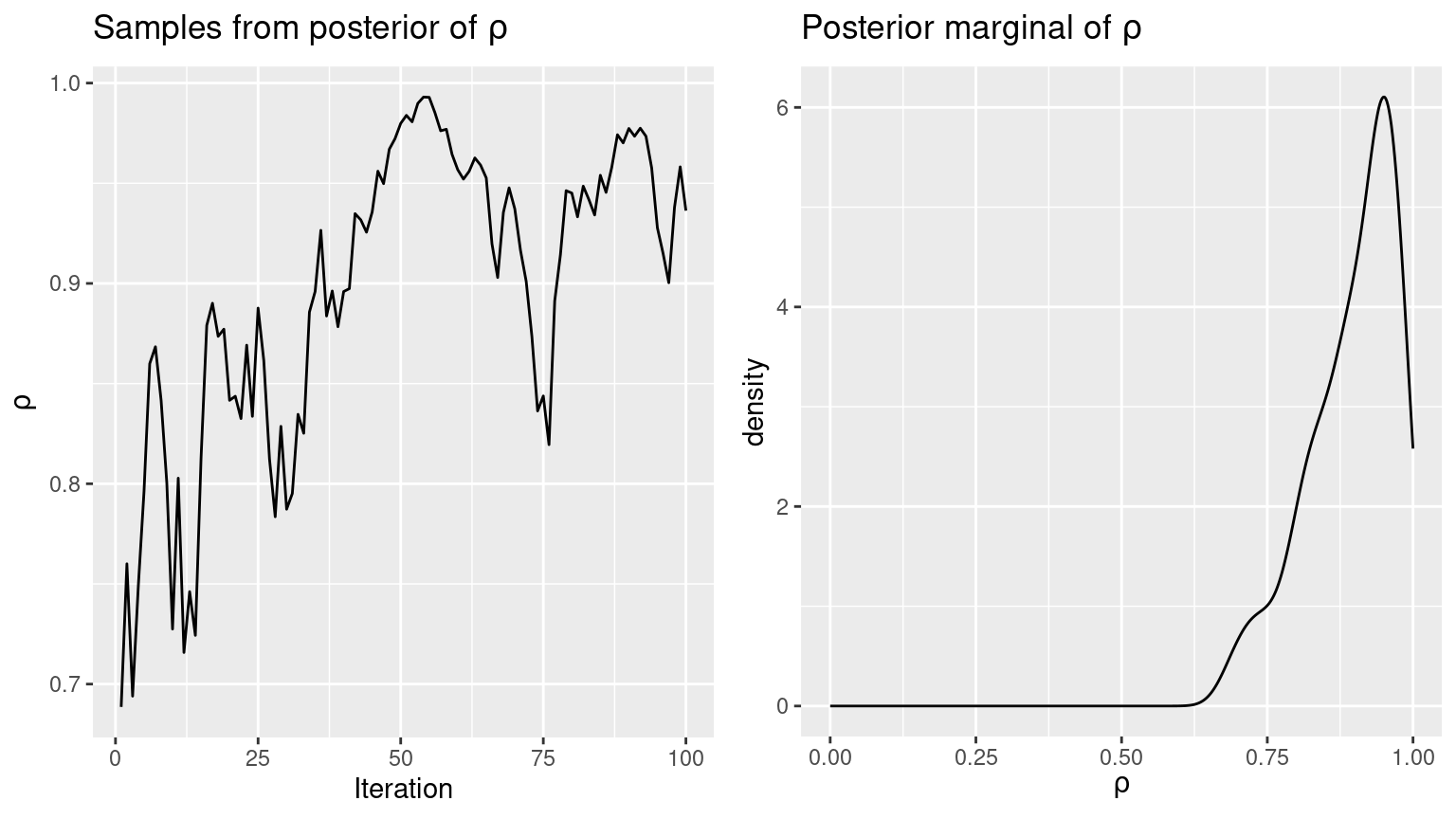
Figure 11.4: Samples from the posterior distribuion (left) and kernel density estimate of the posterior marginal of the spatial autocorrelation parameter.

In addition, summary statistics can be obtained from these samples:

#Posterior mean
mean(rho.sim)

## [1] 0.8956

#Posterior st. dev.
sd(rho.sim)

## [1] 0.07529

#Quantiles
quantile(rho.sim)

##     0%    25%    50%    75%   100% 
## 0.6886 0.8432 0.9157 0.9560 0.9930

Finally, the posterior marginals of all the other parameters of interest can be obtained from the output generated by the INLA within MCMC algorithm. Bayesian model averaging can be used on the conditional marginals and all fitted models are assumed to have the same weight, as these are associated with independent samples from the posterior distribution of \(\rho\).

11.6 Comparison of results

In the previous sections three different methods to implement new latent effects have been described. Figure 11.5 displays the different posterior marginals of \(\rho\) computed using these three different approaches. Marginals obtained with rgeneric and INLA within MCMC are very close, and the one obtained by BMA is not far from those. In all cases, marginals seem to favor values of \(\rho\) very close to the upper bound of its support. This is a well known behavior for the proper CAR model when data have a strong spatial pattern that is not accounted for by the covariates.

Having estimates close to the boundaries of the support of the parameter can be problematic. In particular, BMA may struggle. The reason may be that when the parameter is close to the boundary of its support INLA finds it difficult to obtain accurate estimates of the marginal likelihood required to combine all the conditional models together.

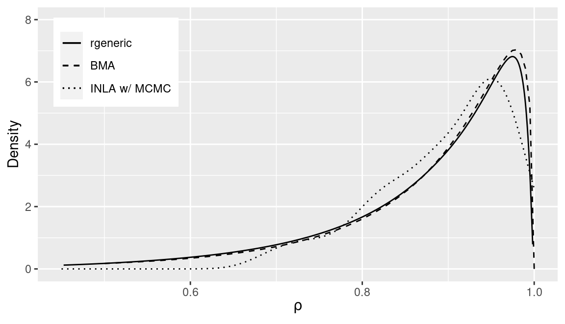
Figure 11.5: Comparison of posterior marginals of the spatial autocorrelation parameter obtained with three different methods.

11.7 Final remarks

In this chapter we have considered three different options to use INLA to fit models with unimplemented latent effects. The rgeneric latent effect provides an adequate way of making computations completely within the INLA package. The other two options, based on BMA and MCMC, are alternative approaches that can be more flexible as to the types of variables that they can handle.

For example, INLA assumes that all hyperparameters are continuous in some interval. BMA and INLA within MCMC can be used to fit models in which the hyperparameters are discrete. This is discussed, for example, in Chapter 13 where fitting mixture models with INLA is considered and Chapter 12, where the imputation of missing covariates is discussed.

In addition, INLA within MCMC can be regarded as a novel way of implementing MCMC algorithms. As seen in the previous sections, it makes implementing MCMC algorithms easy as it focuses in on a small number of hyperparameters and all the others are integrated out by INLA.

Finally, the rgeneric framework can be used to develop multivariate latent random effects. This requires a model with different likelihoods and a definition of the latent effect that works on data in more than one likelihood of the model. Palmí-Perales, Gómez-Rubio, and Martínez-Beneito (2019) show how to implement multivariate latent spatial effects for multivariate spatial data and provide different applications in disease mapping. Similarly, Gómez-Rubio, Cameletti, and Blangiardo (2019) describe how to implement new latent effects to deal with missing values in the covariates and impute them.

References

Banerjee, S., B. P. Carlin, and A. E. Gelfand. 2014. Hierarchical Modeling and Analysis for Spatial Data. 2nd ed. Boca Raton, FL: Chapman & Hall/CRC.

Bivand, Roger S., Virgilio Gómez-Rubio, and HRue. 2014. “Approximate Bayesian Inference for Spatial Econometrics Models.” Spatial Statistics 9: 146–65.

Bivand, Roger S., Virgilio Gómez-Rubio, and Håvard Rue. 2015. “Spatial Data Analysis with R-INLA with Some Extensions.” Journal of Statistical Software 63 (20): 1–31. http://www.jstatsoft.org/v63/i20/.

Gómez-Rubio, Virgilio, Roger S. 2019. “Bayesian model averaging with the integrated nested Laplace approximation.” arXiv E-Prints, November, arXiv:1911.00797. http://arxiv.org/abs/1911.00797.

Gómez-Rubio, Virgilio, Michela Cameletti, and Marta Blangiardo. 2019. “Missing Data Analysis and Imputation via Latent Gaussian Markov Random Fields.” arXiv E-Prints, December, arXiv:1912.10981. http://arxiv.org/abs/1912.10981.

Gómez-Rubio, Virgilio, and HRue. 2018. “Markov Chain Monte Carlo with the Integrated Nested Laplace Approximation.” Statistics and Computing 28 (5): 1033–51.

Haining, Robert. 2003. Spatial Data Analysis: Theory and Practice. Cambridge University Press.

Hoeting, Jennifer, David Madigan, Adrian Raftery, and Chris Volinsky. 1999. “Bayesian Model Averaging: A Tutorial.” Statistical Science 14: 382–401.

Palmí-Perales, Francisco, Virgilio Gómez-Rubio, and Miguel A. Martínez-Beneito. 2019. “Bayesian Multivariate Spatial Models for Lattice Data with INLA.” arXiv E-Prints, September, arXiv:1909.10804. http://arxiv.org/abs/1909.10804.

R Core Team. 2019b. Writing R Extensions. https://cran.r-project.org/doc/manuals/R-exts.html.

Wutzler, Thomas. 2018. Logitnorm: Functions for the Logitnormal Distribution. https://CRAN.R-project.org/package=logitnorm.