Chapter 1 Introduction to Bayesian Inference

1.1 Introduction

Bayesian inference has experienced a boost in recent years due to important advances in computational statistics. This book will focus on the integrated nested Laplace approximation (INLA, Havard Rue, Martino, and Chopin 2009) for approximate Bayesian inference. INLA is one of several recent computational breakthroughs in Bayesian statistics that allows fast and accurate model fitting.

The aim of this introduction is not to provide a thorough introduction to Bayesian inference but to introduce some notation and context for the other chapters of the book. For those readers that may require it, recent introductory texts to Bayesian inference include Kruschke (2015) and McElreath (2016). Both texts cover the basics and provide a good number of examples using a number of programming languages for Bayesian computation. More advanced texts include classics Gelman et al. (2013) and Carlin and Louis (2008), which provide more in depth details on a wide range of topics on Bayesian inference.

1.2 Bayesian inference

In the Bayesian paradigm all unknown quantities in the model are treated as random variables and the aim is to compute (or estimate) the joint posterior distribution. This is, the distribution of the parameters, \(\bm\theta\), conditional on the observed data \(\mathbf{y}\). The way that posterior distribution is obtained relies on Bayes’ theorem:

\[ \pi(\bm\theta \mid \mathbf{y}) = \frac{\pi(\mathbf{y} \mid \bm\theta)\pi(\bm\theta)}{\pi(\mathbf{y})} \]

Here, \(\pi(\mathbf{y} \mid \bm\theta)\) is the likelihood of the data \(\mathbf{y}\) given parameters \(\bm\theta\) (that take values in a parametric space \(\Theta)\), \(\pi(\bm\theta)\) is the prior distribution of the parameters and \(\pi(\mathbf{y})\) is the marginal likelihood, which acts as a normalizing constant. The marginal likelihood is often difficult to compute as it is equal to

\[ \int_{\Theta} \pi(\mathbf{y} \mid \bm\theta)\pi(\bm\theta) d\bm\theta \]

Note that the posterior distribution \(\pi(\bm\theta \mid \mathbf{y})\) is often a highly multivariate distribution and that it is only available in closed form for a few models because the marginal likelihood \(\pi(\mathbf{y})\) is often difficult to estimate. In practice, the posterior distribution is estimated without computing the marginal likelihood. This is why Bayes’ theorem is often stated as

\[ \pi(\bm\theta \mid \mathbf{y}) \propto \pi(\mathbf{y} \mid \bm\theta)\pi(\bm\theta) \]

This means that the posterior can be estimated by re-scaling the product of the likelihood and the prior so that it integrates up to one.

The likelihood of the model describes the data generating process given the parameters, and the prior usually reflects any previous knowledge about the model parameters. When this knowledge is scarce, vague priors are assumed so that the posterior distribution is driven by the observed data.

Summary statistics on the model parameters \(\bm\theta\) can be obtained from the joint posterior distribution \(\pi(\bm\theta \mid \mathbf{y})\). In addition, the posterior marginal distribution of each element of \(\bm\theta\) can be obtained by integrating the remainder of the parameters out:

\[ \pi(\theta_i \mid \mathbf{y}) = \int \pi(\bm\theta \mid \mathbf{y}) d\bm\theta_{-i},\ i=1,\ldots, \textrm{dim}(\bm\theta) \]

Here, \(\theta_{-i}\) represents the set of elements in \(\bm\theta\) minus \(\theta_i\). Posterior marginal distributions are very useful to summarize individual parameters and to compute summary statistics. Important quantities are the posterior mean, standard deviation, mode and quantiles.

1.3 Conjugate priors

As mentioned above, the posterior distribution is only available in closed form for a few models. Models with conjugate priors are those in which the prior is of the same form as the likelihood. For example, if the likelihood is a Gaussian distribution with known precision, the conjugate prior on the mean is a Gaussian distribution. This will ensure that the posterior distribution of the mean is also a Gaussian distribution.

For example, let it be a set of observations \(\{y_i\}_{i=1}^n\) that follow a Gaussian distribution

\[ y_i \mid \mu,\tau \sim N(\mu, \tau),\ i=1,\ldots, n \]

with \(\mu\) the unknown mean and \(\tau\) a known precision. The prior on \(\mu\) can be a Normal distribution with mean \(\mu_0\) and precision \(\tau_0\):

\[ \mu \sim N(\mu_0, \tau_0) \]

The posterior distribution of \(\mu\) (i.e., the distribution of \(\mu\) given data \(\mathbf{y}\)) is \(N(\mu_1,\tau_1)\) with

\[ \mu_1 = \mu_0 \frac{\tau_0}{\tau_0 + \tau n} + \overline{y}\frac{\tau n}{\tau_0 + \tau n} \]

\[ \tau_1 = \tau_0 + n\tau \]

This illustrates Bayesian learning quite well. First of all, the posterior mean is a compromise between the prior mean \(\mu_0\) and the mean of the observed data \(\overline{y}\). When the number of observations is large, then the posterior mean is close to that of the data. If \(n\) is small, more weight is given to our prior belief about the mean. Similarly, the posterior precision is a function of the prior precision and the likelihood precision and it tends to infinity with \(n\), which means that the variance of \(\mu\) tends to zero as the number of data increases.

Other well known conjugate models include the Beta-Binomial model and the Poisson-Gamma model (Gelman et al. 2013).

1.4 Computational methods

When the posterior distribution is not available in a closed form it is necessary to resort to other methods to estimate it or, alternatively, to draw samples from it. Given a sample from the posterior, the Ergodic theorem ensures that moments and other quantities of interest can be estimated (Brooks et al. 2011).

In general, computational methods aim at estimating the integrals that appear in Bayesian inference. For example, the posterior mean of parameter \(\theta_i\) (with values in the parameter space \(\Theta_i\)) is computed as

\[ \int_{\Theta_i} \theta_i \pi(\theta_i \mid \mathbf{y}) d\theta_i \]

Distribution \(\pi(\theta_i \mid \mathbf{y})\) is the marginal posterior distribution of univariate parameter \(\theta_i\). Similarly, the posterior variance or any other moment can be computed as well. Integrals of this type can be conveniently approximated using numerical integration methods and the Laplace approximation (Tierney and Kadane 1986).

Furthermore, typical Monte Carlo methods to sample from densities known up to a constant can be used to obtain samples from the posterior distribution. These methods include rejection sampling and other methods (Carlin and Louis 2008). However, most of these methods will not work well in high dimensional spaces.

Point estimates of the model parameters can be obtained by maximizing the the product of the likelihood and the prior. This is denoted by Maximum A Posteriori (MAP) estimation. Maximization of the posterior distribution is usually performed in the log scaled and it can be effectively achieved using different methods, such as the Newton-Raphson algorithm or the Expectation-Maximization algorithm (Gelman et al. 2013).

1.5 Markov chain Monte Carlo

Markov chain Monte Carlo (MCMC) methods (Gilks et al. 1996; Brooks et al. 2011) are a class of computational methods to draw samples from the joint posterior distribution. These methods are based on constructing a Markov Chain with stationary distribution the posterior distribution. Hence, by sampling from this Markov chain repeatedly, samples from the joint posterior distribution are obtained after a number of iterations.

Several algorithms have been proposed (see Brooks et al. 2011 for a recent summary) but two of them provide a toolbox for Bayesian inference: the Metropolis-Hastings algorithm and Gibbs sampling.

The Metropolis-Hastings algorithm uses a proposal distribution to obtain new values for the ensemble of parameters. This is, given current value \(\bm\theta\) a new value \(\bm\theta^{'}\) is drawn from density \(q(\cdot \mid \bm\theta)\). The proposal distribution can be chosen in many different ways. However, not all proposals will be accepted. When a new proposal is drawn it is accepted with probability

\[ \min\left\{1, \frac{q(\bm\theta \mid \bm\theta^{'})\pi(\bm\theta^{'} \mid \mathbf{y})}{q(\bm\theta^{'} \mid \bm\theta)\pi(\bm\theta \mid \mathbf{y})}\right\} \]

Here, \(q(\bm\theta \mid \bm\theta^{'})\) represents the density of the proposal distribution \(q(\cdot \mid \bm\theta^{'})\) evaluated at \(\bm\theta\). Note also that the acceptance probability contains the posterior distributions to be estimated (and that are unknown). However, the previous acceptance probability can be rewritten as

\[ \min\left\{1, \frac{q(\bm\theta \mid \bm\theta^{'})\pi(\mathbf{y} \mid \bm\theta^{'})\pi(\bm\theta^{'})}{q(\bm\theta^{'} \mid \bm\theta)\pi(\mathbf{y} \mid \bm\theta)\pi(\bm\theta)}\right\} \]

by using Bayes’ rule. Note that now the scaling constant \(\pi(\mathbf{y})\) is not needed to compute the ratio, which is why the Metropolis-Hastings algorithm is so popular.

The ratio essentially ensures that newly proposed values are accepted in the right proportion to be samples from the posterior distribution. In addition, the ratio also will favor moving to new values when there is a high chance of coming back to the current value. This makes sense because this will avoid getting trapped in areas of low posterior probability.

Gibbs sampling (Geman and Geman 1984) can be regarded as a particular case of the Metropolis-Hastings algorithm in which the proposal distributions are the full conditional distribution of the model parameters, i.e., \(\pi(\theta_i \mid \mathbf{y}, \bm\theta_{-i})\). This ensures that the acceptance probability in the Metropolis-Hastings algorithm is always one, which means that all proposals are automatically accepted.

In practice, convergence to the posterior distribution will take a number of iterations, and the first batch of simulations (or burn-in) is discarded for inference. Furthermore, given that samples are often correlated, a thinning is applied to the remaining samples, and many of them will be discarded as well (see, for example, Link and Eaton 2012 and the references therein). Several criteria can be used to assess that the simulation have converged to the stationary state (Gelman and Rubin 1992; Brooks and Gelman 1998).

1.6 The integrated nested Laplace approximation

Havard Rue, Martino, and Chopin (2009) have developed a novel computational method for Bayesian inference. In particular, they focus on estimating the posterior marginals of the model parameters. Hence, instead of estimating a highly multivariate joint posterior distribution \(\pi(\bm\theta \mid \mathbf{y})\) they focus on obtaining approximations to univariate posterior distributions \(\pi(\theta_i \mid \mathbf{y})\). They have termed this approximation the integrated nested Laplace approximation (INLA).

Although the models that INLA can fit are restricted to the class of models that can be expressed as a latent Gaussian Markov random field (Rue and Held 2005), this includes a myriad of commonly used models. In addition, the authors have developed an R package, INLA, for easy model fitting.

1.7 An introductory example: U’s in Game of Thrones books

In order to introduce the different approaches to Bayesian inference outlined above, an introductory example is developed here. Note that the aim is to show where the INLA methodology fits into the Bayesian ecosystem and that some knowledge of Bayesian inference is required to follow the example.

We will consider the average number of u’s on a page of any of the books in the Game of Thrones series. For data collection, only pages from the Preface of each of the five books published by Bantam Books in 2001 were considered. Pages with headers or that were not complete (i.e., had missing lines) were not considered. Data were collected by participants in the 2nd Valencia International Bayesian Summer School (VIBASS2, http://vabar.es) held in Valencia (Spain) in July 2018.

Data is provided in a CSV file that can be loaded and summarized as follows:

GoT <- read.csv2(file = "data/GoT.csv")
summary(GoT)

##        Us      
##  Min.   :15.0  
##  1st Qu.:27.5  
##  Median :31.0  
##  Mean   :33.0  
##  3rd Qu.:36.5  
##  Max.   :62.0

Altogether, there are 31 observations. Because this is a counting process, a Poisson likelihood seems a reasonable choice:

\[ U_i \sim Po(\lambda),\ i=1,\ldots,31 \]

Parameter \(\lambda\) is the mean of the Poisson distribution and the parameter that we are interested in. Remember that the probability distribution of a Poisson is

\[ P(X = x \mid\lambda) = \frac{\exp(-\lambda)\lambda^x}{x!} \]

Note that letter u is not the most common vowel in English, and this fact can be used to make a choice about the prior distribution. Each page has about 20 lines and, say that we are certain that there will be about one or two u’s per line. This prior guess can be used to set a prior on the parameter \(\lambda\).

A Gamma distribution is the conjugate prior for a Poisson likelihood (Gelman et al. 2013). This is defined by two parameters, \(a\) and \(b\), that define the mean, \(a/b\), and variance, \(a/b^2\). The probability density of the Gamma distribution is

\[ f_X(x \mid a, b) = b\exp(-b\cdot x)\frac{(b\cdot x)^{a-1}}{\Gamma(a)} \]

Given our prior guess, we can take a Gamma with mean 30 and variance 5, which gives a high prior probability to \(\lambda\) being between 20 and 40. Hence, the parameters of the prior Gamma distribution are \(a=180\) and \(b=6\).

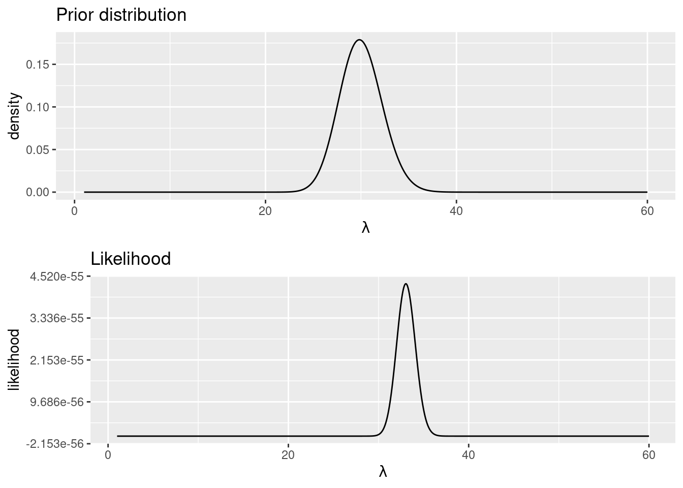
Figure 1.1: Likelihood and prior of the number of u’s on a page of Game of Thrones.

A common way to visualize the likelihood and the prior is to plot them together. Figure 1.1 shows the prior and the likelihood. Note how they are in different scales but the modes are close, which means that our prior guess was not that bad after all. The posterior distribution will be obtained by combining the prior and the likelihood using Bayes’ rule.

The maximum likelihood estimate is simply the mean of the data:

mean(GoT$Us)

## [1] 33.03

The Maximum A Posteriori (MAP) estimate can be obtained by maximizing the sum of the log-prior and the log-likelihood:

got.logposterior <- function(lambda) {
  dgamma(lambda, 180, 6, log = TRUE) + sum(dpois(GoT$Us, lambda,
    log = TRUE))
}

#Maximize log-posterior
got.MAP <- optim(30, got.logposterior, control = list(fnscale = -1))
got.MAP$par

## [1] 32.51

Given that the Gamma distribution is conjugate for a Poisson likelihood, the posterior is available in a closed form, and it is a Gamma with parameters \(a + \sum_{i=1}^{31} U_i\) and \(b + n\). The posterior distribution has been plotted in Figure 1.2.

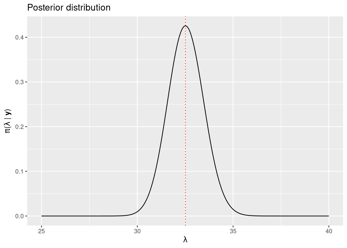
Figure 1.2: Posterior distribution of the number of u’s in a book of Game of Thrones using a conjugate prior (black solid line) and MAP estimate (dotted red line).

A Metropolis-Hastings algorithm to estimate the posterior distribution of the parameter \(\lambda\) can be implemented in this case. As a proposal density we will consider a log-Normal distribution centered at the current value of the mean \(\lambda\) and with small standard deviation equal to \(0.05\).

The algorithm will obtain 2100 values of \(\lambda\), starting at 20:

n.sim <- 2100
lambda <- rep(NA, n.sim)
lambda[1] <- 20

The implementation of the Metropolis-Hastings algorithm is the following:

set.seed(1)
for (i in 2:n.sim) {
  # Draw new value
  lambda.new <- rlnorm(1, log(lambda[i - 1]), 0.05)

  #Log-acceptance probability
  acc.prob <- dlnorm(lambda[i -1], log(lambda.new), 0.05, log = TRUE) + 
    dgamma(lambda.new, 180, 6, log = TRUE) +
    sum(dpois(GoT$Us, lambda.new, log = TRUE)) -
    dlnorm(lambda.new, log(lambda[i - 1]), 0.05, log = TRUE) -
    dgamma(lambda[i - 1], 180, 6, log = TRUE) -
    sum(dpois(GoT$Us, lambda[i - 1], log = TRUE))

  acc.prob <- min(1, exp(acc.prob))

  # Accept/reject new value  
  if(runif(1) < acc.prob) {
    lambda[i] <- lambda.new
  } else {
    lambda[i] <- lambda[i -1]
  }

}

Figure 1.3 shows the samples of \(\lambda\) obtained with the Metropolis-Hastings algorithm. The first iterations provide values that are too close to the initial value and these are often taken as a burn-in and discarded. The remaining values are used for inference. However, given that they seem a bit correlated it is usual to conduct a thinning on them. In this case, 100 iterations will be taken as burn-in, and thinning will be done on the remaining observations, so that only one in five is kept. As a result, there will be 400 values for inference.

Removing the burn-in iterations and thinning can be done as follows:

lambda2 <- lambda[seq(101, n.sim, by = 5)]

Summary statistics of the posterior distribution of \(\lambda\) can be obtained by taking summary statistics on the sampled values:

summary(lambda2)

##    Min. 1st Qu.  Median    Mean 3rd Qu.    Max. 
##    30.0    32.0    32.7    32.6    33.2    36.2

Kernel density can be used to obtain an estimate of the posterior marginal distribution of \(\lambda\) from the final set of values. This is shown in the plot at the bottom in Figure 1.3. It is worth mentioning that the estimates obtained with the Metropolis-Hastings algorithm are very close to those obtained with the other methods computed so far because we are actually fitting the same model. Any differences are due to the Monte Carlo error inherent to MCMC methods, but this error can usually be reduced by increasing the number of samples drawn. In any case, we provide a comparison and summary of the different estimates obtained at the end of this section.

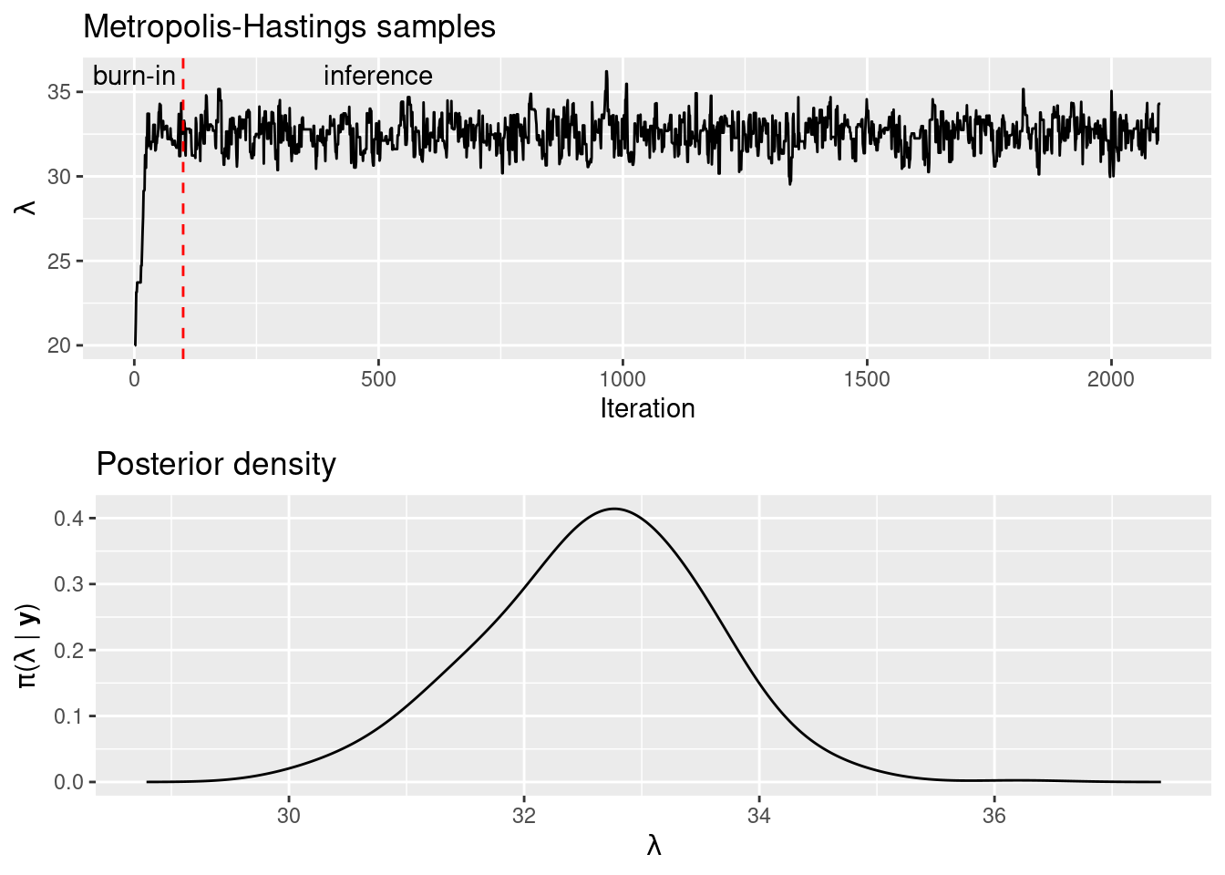
Figure 1.3: Samples of \(\lambda\) obtained with the Metropolis-Hastings algorithm (top) and kernel density estimate of the posterior distribution using the samples (bottom).

Finally, we show how to fit these models using INLA. First of all, the model fit will be the following:

\[ U_i \sim Po(\lambda),\ i=1,\ldots, 31 \]

\[ \log(\lambda) = \alpha \]

\[ \pi(\alpha) \propto 1 \]

Parameter \(\alpha\) is the intercept of the linear predictor and it is assigned a constant prior. This is an improper prior because it does not integrate to one but these are sometimes useful to provide a vague prior. Note that \(\lambda\) is not modeled directly but in the log-scale through the intercept of the linear predictor \(\alpha\). This model can be implemented with INLA using the following code (that will not be discussed here in detail):

GoT.inla <- inla(Us ~ 1, data = GoT, family = "poisson",
  control.predictor = list(compute = TRUE)
) 

Summary statistics of the posterior distribution of \(\alpha\) are:

GoT.inla$summary.fixed

##              mean      sd 0.025quant 0.5quant 0.975quant  mode       kld
## (Intercept) 3.498 0.03127      3.436    3.498      3.558 3.498 4.908e-07

The posterior distribution of \(\lambda\) can be obtained by transforming the posterior distribution of \(\alpha\) given that \(\lambda = \exp(\alpha)\) (see Section 2.6):

marg.lambda <- inla.tmarginal(exp, GoT.inla$marginals.fixed[[1]])
inla.est <- inla.zmarginal(marg.lambda)

## Mean            33.049 
## Stdev           1.02682 
## Quantile  0.025 31.059 
## Quantile  0.25  32.3464 
## Quantile  0.5   33.0376 
## Quantile  0.75  33.7378 
## Quantile  0.975 35.0904

In order to compare the different approaches, we have produced Table 1.2 that includes estimates based on the methods described so far. In this case, point estimates of parameter \(\lambda\) are very similar. Note also that the maximum likelihood estimate is very close to the posterior modes obtained with all Bayesian methods. The point estimates of the posterior standard deviation are also very similar among the three Bayesian methods that computed them. The quantiles computed are also very close. It is worth mentioning that in this particular case the mode is simple and we have enough data to estimate the only parameter in the model. Hence, it would be expected that all results should be similar.

Table 1.1: Table: Table 1.2: Summary of estimates using different Bayesian estimation methods.

Method	Mean	Mode	St. dev.	0.025 quant.	0.975 quant.
Max. lik.	NA	33.03	NA	NA	NA
MAP	NA	32.51	NA	NA	NA
Conjugate	32.54	32.51	0.9378	30.73	34.40
M-H	32.47	32.77	1.2625	30.55	34.33
INLA	33.05	33.02	1.0268	31.06	35.09

Table: (#tab:GoTestimates) Summary of estimates using different Bayesian estimation methods.

Figure 1.4 shows the different estimates of the posterior marginal and MAP estimate of parameter \(\lambda\) obtained with the different methods presented here. As we had seen previously, all methods provide very similar estimates of the posterior marginal. Note that for more complex models it may simply not be possible to obtain the marginals in a closed form and that estimation will most often rely on MCMC or INLA methods.

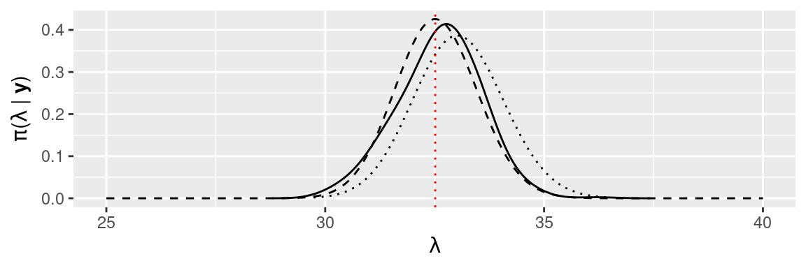
Figure 1.4: Comparison of the different estimates of the posterior marginal of \(\lambda\) provided by the methods described in this chapter: MCMC (solid line), conjugate prior (dashed line), INLA (dotted line) and MAP (vertical red dotted line).

1.8 Final remarks

As stated at the beginning of this chapter, the aim is to provide an introduction to Bayesian inference. In particular, to provide some context so that readers can place the integrated nested Laplace approximation within the Bayesian ecosystem. This is important for many reasons. First of all, INLA is one of many ways to make Bayesian inference. INLA may be the right approach in many occasions, but it might simply be the wrong approach on some other occasions. Secondly, this also means that having a deep knowledge of INLA is useful to identify models where it will work well and other where it will perform badly.

Chapter 2 introduces the integrated nested Laplace approximation methodology and the use of the INLA package for Bayesian model fitting. A number of latent effects for model building are described in Chapter 3. Next, multilevel models are tackled in Chapter 4. Prior distributions are summarized in Chapter 5. Additional features that can be used to fit more complex models are detailed in Chapter 6. Different types of models with spatial dependence are depicted in Chapter 7. The analysis of time series by means of temporally correlated models and spatio-temporal models are presented in Chapter 8. Splines and other smoothing methods are described in Chapter 9. The analysis of time-to-event data using survival and joint models is examined in Chapter 10. Different ways of fitting new models not implemented in the INLA package are illustrated in Chapter 11. Handling missing values in both the response and covariates is described in Chapter 12. Finally, the analysis of mixture models with INLA is explained in Chapter 13.

References

Brooks, S. P., and A. Gelman. 1998. “General Methods for Monitoring Convergence of Iterative Simulations.” Journal of Computational and Graphical Statistics 7: 434–55.

Brooks, Steve, Andrew Gelman, Galin L. Jones, and Xiao-Li Meng. 2011. Handbook of Markov Chain Monte Carlo. Boca Raton, FL: Chapman & Hall/CRC Press.

Carlin, Bradley P., and Thomas A. Louis. 2008. Bayesian Methods for Data Analysis. 3rd ed. Boca Raton, FL: Chapman & Hall/CRC Press.

Gelman, Andrew, John B. Carlin, Hal S. Stern, David B. Dunson, Aki Vehtari, and Donald B. Rubin. 2013. Bayesian Data Analysis. 3rd ed. Boca Raton, FL: Chapman & Hall/CRC Press.

Gelman, A., and D. B. Rubin. 1992. “Inference from Iterative Simulation Using Multiple Sequences.” Statistical Science 7: 457–511.

Geman, S., and D. Geman. 1984. “Stochastic Relaxation, Gibbs Distributions, and the Bayesian Restoration of Images.” IEEE Transactions on Pattern Analysis and Machine Intelligence 6 (6): 721–41.

Gilks, W. R., W. R. Gilks, S. Richardson, and D. J. Spiegelhalter. 1996. Markov Chain Monte Carlo in Practice. Boca Raton, Florida: Chapman & Hall.

Kruschke, John K. 2015. Doing Bayesian Data Analysis, Second Edition: A Tutorial with R, JAGS, and Stan. 2nd ed. Amsterdam: Academic Press.

Link, William A., and Mitchell J. Eaton. 2012. “On Thinning of Chains in MCMC.” Methods in Ecology and Evolution 3 (1): 112–15. https://doi.org/10.1111/j.2041-210X.2011.00131.x.

McElreath, Richard. 2016. Statistical Rethinking: A Bayesian Course with Examples in R and Stan. Boca Raton, FL: Chapman & Hall/CRC Press.

Rue, Havard, Sara Martino, and Nicolas Chopin. 2009. “Approximate Bayesian Inference for Latent Gaussian Models by Using Integrated Nested Laplace Approximations.” Journal of the Royal Statistical Society, Series B 71 (2): 319–92.

Rue, H., and L. Held. 2005. Gaussian Markov Random Fields: Theory and Applications. Chapman; Hall/CRC Press.

Tierney, Luke, and Joseph B. Kadane. 1986. “Accurate Approximation for Posterior Moments and Marginal Densities.” Journal of the Americal Statistical Association 81 (393): 82–86.