Chapter 6 Advanced Features

6.1 Introduction

As seen in previous chapters, INLA is a methodology to fit Bayesian hierarchical models by computing approximations of the posterior marginal distributions of the model parameters. In order to build more complex models and compute the posterior marginal distribution of some quantities of interest, the INLA package has a number of advanced features that are worth knowing. Some of these features are also described in detail in Krainski et al. (2018).

In this chapter we will describe some of these features. In particular, Section 6.2 shows how to define a predictor matrix that multiplies all terms in the linear predictor, so that the actual linear predictor of the model is a linear combination of the effects in the model formula. Next, Section 6.3 presents how to define linear combinations of the latent effects to compute their posterior distribution. Section 6.4 introduces the use of models with several likelihoods. Models with several likelihoods that share some terms are in Section 6.5, where the copy and replicate features are described in detail. These features are very useful when working with, for example, joint models (see Chapter 10).

6.2 Predictor Matrix

The formula passed to the inla() function defines the model to be fit by INLA, i.e., the formula defines the terms in the linear predictor. However, sometimes we need to modify the model so that linear combinations of these terms are used instead of simply the ones set in the formula. INLA allows this by defining a matrix A, which is called predictor matrix so that the actual linear predictor \(\bm\eta^*\) used is

\[ \bm\eta^* = A \bm\eta \]

Here, \(\bm\eta\) is the linear predictor defined in the formula. By default, this matrix is the identity matrix.

Matrix A that defines the linear combinations to be used is passed using element A in the list passed to argument control.predictor (see Section 2.5 for details). Matrix A can be a dense matrix or a sparse one of the types implemented in the Matrix package (Bates and Maechler 2019). The dimension of the A matrix must be \(n\times n\), with \(n\) the number of observations in the model.

In order to provide a simple example we will consider the cement dataset described in Section 2.3. A very simple use of the A matrix is to re-scale the linear predictor used in the model (see Krainski et al. 2018 for a similar example), for example, to have it multiplied by a constant. In this case, we will take the A matrix as a diagonal matrix with values equal to 5. This means that the linear predictors, as defined by the formula, will be multiplied by 5, and that the estimates of the terms in the linear predictor will shrink in a similar way so that the actual linear predictor \(A \bm\eta\) remains the same as in the example in Section 2.3. Note that the fitted values will also remain the same.

library("MASS")
library("Matrix")

data(cement)
A <- Diagonal(n = nrow(cement), x = 5)
summary(A)

## 13 x 13 diagonal Matrix of class "ddiMatrix" 
##    Min. 1st Qu.  Median    Mean 3rd Qu.    Max. 
##       5       5       5       5       5       5

Note how in the code above matrix A is a sparse matrix. Hence, the model using this predictor matrix can be fit:

m1.A <- inla(y ~ x1 + x2 + x3 + x4, data = cement,
  control.predictor = list(A = A))
summary(m1.A)

## 
## Call:
##    "inla(formula = y ~ x1 + x2 + x3 + x4, data = cement, 
##    control.predictor = list(A = A))" 
## Time used:
##     Pre = 0.422, Running = 0.0601, Post = 0.0262, Total = 0.508 
## Fixed effects:
##               mean     sd 0.025quant 0.5quant 0.975quant   mode kld
## (Intercept) 12.482 13.997    -15.556   12.481     40.495 12.482   0
## x1           0.310  0.149      0.012    0.310      0.608  0.310   0
## x2           0.102  0.145     -0.188    0.102      0.391  0.102   0
## x3           0.020  0.151     -0.282    0.020      0.322  0.020   0
## x4          -0.029  0.142     -0.313   -0.029      0.255 -0.029   0
## 
## Model hyperparameters:
##                                          mean    sd 0.025quant 0.5quant
## Precision for the Gaussian observations 0.209 0.093      0.068    0.195
##                                         0.975quant  mode
## Precision for the Gaussian observations      0.428 0.167
## 
## Expected number of effective parameters(stdev): 5.00(0.00)
## Number of equivalent replicates : 2.60 
## 
## Marginal log-Likelihood:  -67.60

Note how the estimates of the fixed effects are divided by 5 as compared to the estimates obtained with the model fit in Section 2.3. This is because of the effect of the A matrix.

In general, the predictor matrix can be useful for non-trivial examples. For example, the predictor matrix plays an important role in the development of spatial models based on stochastic partial differential equations (Krainski et al. 2018). See Chapter 7 for details.

6.3 Linear combinations

The use of the predictor matrix introduced in the previous section allows us to define models where the actual linear predictors are linear combinations of the effects in the model formula. However, in some situations we are only interested in computing linear combinations on some effects without altering model fitting.

With INLA, linear combinations on the different latent effects can be defined and their posterior marginals estimated. Note that these linear combinations do not alter the fit model (as the use of a predictor matrix did). Linear combinations are passed using argument lincomb to the inla() function. Furthermore, argument control.lincomb can be used to set the parameters that control how posterior marginals of linear combinations are computed. Table 6.1 shows the options available to control how the linear combinations are fit.

Table 6.1: Summary of options in `control.lincomb`.
Argument	Default	Description
`precision`	`1e09`	Tiny noise added to compute approximation
`verbose`	`TRUE`	Use verbose if verbose is enabled globally.

Linear combinations are defined by setting the effects and the associated coefficients that they have to make the linear combination. Two functions are available to define linear combinations: inla.make.lincomb(), to define a single linear combination, and inla.make.lincombs(), to define several linear combinations at once.

Function inla.make.lincomb() takes named arguments with the values of the coefficients of the linear combination. The names are the names of the effects to be used in the linear combination. For fixed effects, values must be a single number, while for random effects it is a vector of coefficients of the same length as the index of the random effect. For those values of the random effect not in the linear combination, NA must be used.

For example, in the analysis of the cement data above we might be interested in computing the difference between coefficients of covariates x1 and x2. This could be defined as follows:

inla.make.lincomb(x1 = 1, x2 = -1)

If the linear combination involves a random effect index from 1 to \(p\), the linear combination can be defined by including a term with the name of the latent random effect. The value now is not a single number, but a vector of length \(p\) with the coefficients of the different elements of the random effects. Those elements that do not appear in the linear combination must have a value of NA.

For example, if a random effect named u of length 4 is included in a model and we want to compute the difference between its two terms, this can be set up as:

inla.make.lincomb(u = c(1, -1, NA, NA))

Function inla.make.lincombs() can be used to set more than one linear combination at a time. Instead of using a single value for the linear combinations on the fixed effects, a vector of coefficients can be passed.

For example, say that we are interested in comparing the coefficient of variable x1 to the other three coefficients. In the design of experiments literature these types of comparisons are often referred to as contrasts. This can be set as several differences using linear combinations as follows:

inla.make.lincomb(
  x1 = c( 1,  1,  1),
  x2 = c(-1,  0,  0),
  x3 = c( 0, -1,  0),
  x4 = c( 0,  0, -1)
)

Once the model has been fit, summaries of the linear combinations are available in summary.lincomb.derived in the inla object returned. Similarly, posterior marginals densities are available in marginals.lincomb.

Finally, two arguments can be passed through control.inla to control how linear combinations are computed: lincomb.derived.only and lincomb.derived.correlation.matrix. The first option indicates whether the linear combinations are to be computed, and the second controls the computation of the correlation matrix of the linear combinations. See Table 6.2 for a summary.

Table 6.2: Options in `control.inla` to control how the linear combinations are computed.
Argument	Default	Description
`lincomb.derived.only`	`TRUE`	Compute full graph of derived linear combinations.
`lincomb.derived.correlation.matrix`	`FALSE`	Compute correlations for derived linear combinations.

Linear combinations can be used for a number of issues, such as computing the posterior marginal of the linear predictor for a given set of covariate values. Another interesting application is to compare whether two effects are equal.

In order to provide a simple example, we will consider the abrasion dataset (Davies 1954) from package faraway (Faraway 2016). This dataset records data from an industrial experiment about wear of four different types of materials after being fed into a wear testing machine. In each run, four samples are processed, and the position of the samples may be important. The different variables in this dataset are described in Table 6.3.

Table 6.3: Variables in the `abrasion` dataset.
Variable	Description
`run`	Run number (from 1 to 4).
`position`	Position number (from 1 to 4).
`material`	Type of material (A, B, C or D).
`wear`	Weight loss (in 0.1mm) over testing period.

Given that the main interest is in the wear depending on the type of material, material will be introduced into the model as a fixed effect, while run and position are introduced as iid random affects. In addition, we have noticed that default INLA priors produce too much shrinkage of the coefficients and random effects towards zero, and the results do not reproduce those in Faraway (2006). In particular, we have considered a larger precision on the coefficients of the fixed effects. For the prior on the precisions we have followed J. J. Faraway (2019 b) and taken a Gamma prior with parameters 0.5 and 95. This is an informative prior that has a mean value half the variance of the residuals of a linear regression on wear using material as predictor. The posterior means of precisions of the random effects should be lower than this value. Furthermore, function inla.hyperpar() has been used to obtain better estimates of the hyperparameters once the model has been fit with INLA.

library("faraway")
data(abrasion)

# Prior prec. of random effects
prec.prior <- list(prec = list(param = c(0.5, 95)))
# Model formula
f.wear <- wear ~ -1 + material + 
    f(position, model = "iid", hyper = prec.prior) +
    f(run, model = "iid", hyper = prec.prior)

# Model fitting
m0 <- inla(f.wear, data = abrasion,
  control.fixed = list(prec = 0.001^2)
)
# Improve estimates of hyperparameters
m0 <- inla.hyperpar(m0)
summary(m0)

## 
## Call:
##    "inla(formula = f.wear, data = abrasion, control.fixed = list(prec 
##    = 0.001^2))" 
## Time used:
##     Pre = 0.241, Running = 1.64, Post = 0.0965, Total = 1.98 
## Fixed effects:
##            mean    sd 0.025quant 0.5quant 0.975quant  mode kld
## materialA 265.7 9.784      246.0    265.7      285.3 265.7   0
## materialB 219.9 9.784      200.3    219.9      239.5 219.9   0
## materialC 241.7 9.784      222.0    241.7      261.3 241.7   0
## materialD 230.4 9.784      210.8    230.4      250.0 230.4   0
## 
## Random effects:
##   Name     Model
##     position IID model
##    run IID model
## 
## Model hyperparameters:
##                                          mean    sd 0.025quant 0.5quant
## Precision for the Gaussian observations 0.022 0.011      0.006    0.020
## Precision for position                  0.008 0.006      0.001    0.006
## Precision for run                       0.010 0.008      0.001    0.008
##                                         0.975quant  mode
## Precision for the Gaussian observations      0.048 0.016
## Precision for position                       0.025 0.004
## Precision for run                            0.030 0.004
## 
## Expected number of effective parameters(stdev): 9.28(0.43)
## Number of equivalent replicates : 1.72 
## 
## Marginal log-Likelihood:  -98.70

Then, we may be interested in comparing whether there is any difference between material A and any of the others. For example, the following linear constraint will compute the difference of the effects between material A and B:

lc <- inla.make.lincomb(materialA = 1, materialB = -1)

This model can now be fit to compare materials A and B:

m0.lc <- inla.hyperpar(inla(f.wear, data = abrasion, lincomb = lc,
  control.fixed = list(prec = 0.001^2)))
summary(m0.lc)

## 
## Call:
##    "inla(formula = f.wear, data = abrasion, lincomb = lc, 
##    control.fixed = list(prec = 0.001^2))" 
## Time used:
##     Pre = 0.258, Running = 1.98, Post = 0.124, Total = 2.36 
## Fixed effects:
##            mean    sd 0.025quant 0.5quant 0.975quant  mode kld
## materialA 265.7 9.784      246.0    265.7      285.3 265.7   0
## materialB 219.9 9.784      200.3    219.9      239.5 219.9   0
## materialC 241.7 9.784      222.0    241.7      261.3 241.7   0
## materialD 230.4 9.784      210.8    230.4      250.0 230.4   0
## 
## Linear combinations (derived):
##    ID  mean    sd 0.025quant 0.5quant 0.975quant  mode kld
## lc  1 45.75 5.455      34.78    45.75      56.73 45.75   0
## 
## Random effects:
##   Name     Model
##     position IID model
##    run IID model
## 
## Model hyperparameters:
##                                          mean    sd 0.025quant 0.5quant
## Precision for the Gaussian observations 0.022 0.011      0.006    0.020
## Precision for position                  0.008 0.006      0.001    0.006
## Precision for run                       0.010 0.008      0.001    0.008
##                                         0.975quant  mode
## Precision for the Gaussian observations      0.048 0.016
## Precision for position                       0.025 0.004
## Precision for run                            0.030 0.004
## 
## Expected number of effective parameters(stdev): 9.28(0.43)
## Number of equivalent replicates : 1.72 
## 
## Marginal log-Likelihood:  -98.70

Note that summary statistics of the posterior marginal of the linear combination can be accessed with

m0.lc$summary.lincomb.derived

##    ID  mean    sd 0.025quant 0.5quant 0.975quant  mode kld
## lc  1 45.75 5.455      34.78    45.75      56.73 45.75   0

This shows a positive posterior means and 95% credible interval that is above 0, which means that wear in material A is higher than in material B.

This can be extended to compare material A to all the other materials. This can be represented by a \(3\times 4\) matrix to represent the 3 linear combinations required. Now inla.make.lincombs must be used in order to define 3 different linear combinations.

lcs <- inla.make.lincombs(
  materialA = c( 1,  1,  1),
  materialB = c(-1,  0,  0),
  materialC = c( 0, -1,  0),
  materialD = c( 0,  0, -1)
)

The model is fit similarly to the previous example:

m0.lcs <- inla.hyperpar(inla(f.wear, data = abrasion, lincomb = lcs,
  control.fixed = list(prec = 0.001^2)))
summary(m0.lcs)

## 
## Call:
##    "inla(formula = f.wear, data = abrasion, lincomb = lcs, 
##    control.fixed = list(prec = 0.001^2))" 
## Time used:
##     Pre = 0.261, Running = 2.58, Post = 0.0931, Total = 2.94 
## Fixed effects:
##            mean    sd 0.025quant 0.5quant 0.975quant  mode kld
## materialA 265.7 9.784      246.0    265.7      285.3 265.7   0
## materialB 219.9 9.784      200.3    219.9      239.5 219.9   0
## materialC 241.7 9.784      222.0    241.7      261.3 241.7   0
## materialD 230.4 9.784      210.8    230.4      250.0 230.4   0
## 
## Linear combinations (derived):
##     ID  mean    sd 0.025quant 0.5quant 0.975quant  mode kld
## lc1  1 45.75 5.455      34.78    45.75      56.73 45.75   0
## lc2  2 24.00 5.455      13.03    24.00      34.98 24.00   0
## lc3  3 35.25 5.455      24.28    35.25      46.23 35.25   0
## 
## Random effects:
##   Name     Model
##     position IID model
##    run IID model
## 
## Model hyperparameters:
##                                          mean    sd 0.025quant 0.5quant
## Precision for the Gaussian observations 0.022 0.011      0.006    0.020
## Precision for position                  0.008 0.006      0.001    0.006
## Precision for run                       0.010 0.008      0.001    0.008
##                                         0.975quant  mode
## Precision for the Gaussian observations      0.048 0.016
## Precision for position                       0.025 0.004
## Precision for run                            0.030 0.004
## 
## Expected number of effective parameters(stdev): 9.28(0.43)
## Number of equivalent replicates : 1.72 
## 
## Marginal log-Likelihood:  -98.70

Linear combinations can also be used to compare the levels of the random effects. For example, let’s consider a comparison between positions 1 and 2. Variable position is an iid random effect with four different levels, and the weights must be set in a vector of the same length. For those levels that must be ignored in the linear combination, NA can be used.

Hence, to define a linear combination to compare levels 1 and 2 of variable position we can define the linear combination as follows:

lc.pos <- inla.make.lincomb(position = c(1, -1, NA, NA))

m0.pos <- inla.hyperpar(inla(f.wear, data = abrasion, lincomb = lc.pos,
  control.fixed = list(prec = 0.001^2)))
summary(m0.pos)

## 
## Call:
##    "inla(formula = f.wear, data = abrasion, lincomb = lc.pos, 
##    control.fixed = list(prec = 0.001^2))" 
## Time used:
##     Pre = 0.247, Running = 1.88, Post = 0.0957, Total = 2.22 
## Fixed effects:
##            mean    sd 0.025quant 0.5quant 0.975quant  mode kld
## materialA 265.7 9.784      246.0    265.7      285.3 265.7   0
## materialB 219.9 9.784      200.3    219.9      239.5 219.9   0
## materialC 241.7 9.784      222.0    241.7      261.3 241.7   0
## materialD 230.4 9.784      210.8    230.4      250.0 230.4   0
## 
## Linear combinations (derived):
##    ID   mean    sd 0.025quant 0.5quant 0.975quant   mode kld
## lc  1 -23.34 5.504     -33.67   -23.59     -11.62 -24.09   0
## 
## Random effects:
##   Name     Model
##     position IID model
##    run IID model
## 
## Model hyperparameters:
##                                          mean    sd 0.025quant 0.5quant
## Precision for the Gaussian observations 0.022 0.011      0.006    0.020
## Precision for position                  0.008 0.006      0.001    0.006
## Precision for run                       0.010 0.008      0.001    0.008
##                                         0.975quant  mode
## Precision for the Gaussian observations      0.048 0.016
## Precision for position                       0.025 0.004
## Precision for run                            0.030 0.004
## 
## Expected number of effective parameters(stdev): 9.28(0.43)
## Number of equivalent replicates : 1.72 
## 
## Marginal log-Likelihood:  -98.70

Fixed and random effects can be combined together to create more complex linear combinations. For example, the following linear combination considers the sum of the effect of material A, position 1 and run 2:

lc.eff <- inla.make.lincomb(materialA = 1, position = c(1, NA, NA, NA),
  run = c(NA, 1, NA, NA))
m0.eff <- inla.hyperpar(inla(f.wear, data = abrasion, lincomb = lc.eff,
  control.fixed = list(prec = 0.001^2)))
summary(m0.eff)

## 
## Call:
##    "inla(formula = f.wear, data = abrasion, lincomb = lc.eff, 
##    control.fixed = list(prec = 0.001^2))" 
## Time used:
##     Pre = 0.248, Running = 1.82, Post = 0.101, Total = 2.17 
## Fixed effects:
##            mean    sd 0.025quant 0.5quant 0.975quant  mode kld
## materialA 265.7 9.784      246.0    265.7      285.3 265.7   0
## materialB 219.9 9.784      200.3    219.9      239.5 219.9   0
## materialC 241.7 9.784      222.0    241.7      261.3 241.7   0
## materialD 230.4 9.784      210.8    230.4      250.0 230.4   0
## 
## Linear combinations (derived):
##    ID mean    sd 0.025quant 0.5quant 0.975quant  mode kld
## lc  1  254 5.906      242.6    253.9      266.3 253.6   0
## 
## Random effects:
##   Name     Model
##     position IID model
##    run IID model
## 
## Model hyperparameters:
##                                          mean    sd 0.025quant 0.5quant
## Precision for the Gaussian observations 0.022 0.011      0.006    0.020
## Precision for position                  0.008 0.006      0.001    0.006
## Precision for run                       0.010 0.008      0.001    0.008
##                                         0.975quant  mode
## Precision for the Gaussian observations      0.048 0.016
## Precision for position                       0.025 0.004
## Precision for run                            0.030 0.004
## 
## Expected number of effective parameters(stdev): 9.28(0.43)
## Number of equivalent replicates : 1.72 
## 
## Marginal log-Likelihood:  -98.70

6.4 Several likelihoods

So far, we have considered models with a single likelihood but INLA can handle models with more than one likelihood. This is useful to define joint models (see Chapter 10) in which one likelihood models survival time and the second one models longitudinal data. The first likelihood will be that of a survival model, while the second one will be of the types used to model longitudinal data.

When using several likelihoods data must be stored in a very particular way. First of all, the response variable must be a matrix with as many columns as likelihoods. Hence, the first column will be the response used by the first likelihood and so on. Data must be stored so that there is one variable per column and a single value of any of the variables per row. All the empty elements in the matrix are set to NA.

For example, let us consider a joint model with response variables \(\mathbf{y} = (y_1\ldots, y_n)\) and \(\mathbf{z} = (z_1,\ldots, z_m)\). Then, data must be stored in a matrix like the following:

\[ \left[ \begin{array}{cc} y_1 & \mathtt{NA}\\ \vdots & \mathtt{NA}\\ y_n & \mathtt{NA}\\ \mathtt{NA} & z_1\\ \mathtt{NA} & \vdots\\ \mathtt{NA} & z_m\\ \end{array} \right] \]

Note that the dimension of this matrix is \((n + m) \times 2\), i.e., the number of rows is the total number of observations and the number of columns is equal to the number of variables. This can be easily generalized to any number of response variables.

When multiple likelihoods are used in a model, these are passed in a vector to argument family. For example, the following code could be used to fit a model with a Gaussian and a Poisson likelihood:

family = c("gaussian", "poisson")

As stated above, the response variables need to be formatted in a particular way. A matrix with as many likelihoods as columns is required. The number of rows is the total number of observations for all likelihoods. If in the example above there are 30 observations from a Gaussian likelihood and 20 from a Poisson one, then the response must be a matrix with 2 columns and 50 rows.

Then, observations are stacked in a matrix so that the observations from the Gaussian likelihood are in the first column and rows 1 to 30. Then, observations for the Poisson likelihood are in the second column and rows 31 to 50. All the other elements in the matrix are filled with NA. This ensures that every row has only a single observed value. Note that then there is an implicit index from 1 to 50 to identify each one of the observations, regardless of the likelihood they belong to.

In order to define the model, all terms for both likelihoods need to be included in the linear predictor. Hence, when defining indices for the latent random effects, this can go (for example) from 1 to the total number of rows in the response matrix. When a covariate only affects observations in a single likelihood, the values for the observations in the other likelihoods must be set to NA. Similarly, the indices of the latent random effects must be set to NA for those observations that do not depend on the latent random effect.

6.4.1 Simulated example

To illustrate the use of several likelihoods we will develop an example here using two (independent) variables from a Gaussian and Poisson likelihood, respectively. First of all, 30 observations from a standard Gaussian distribution and 20 observations from a Poisson with mean 10 will be drawn:

set.seed(314)
# Gaussian data
d1 <- rnorm(30)

# Poisson data
d2 <- rpois(20, 10)

Next, the two response variables will be put in a 2-column matrix as required by INLA:

# Data
d <- matrix(NA, ncol = 2, nrow = 30 + 20)
d[1:30, 1] <- d1
d[30 + 1:20, 2] <- d2

In order to have two different intercepts in the model it is necessary to add them as two separate covariates. In this case, both intercepts have all values equal to one, but the same principle would apply when two separate coefficients are required for the same covariate or when random effects only apply to data in one the likelihoods. Values NA mean that the covariate does not appear in the linear predictor of the response.

# Define a different intercept for each likelihood
Intercept1 <- c(rep(1, 30), rep(NA, 20))
Intercept2 <- c(rep(NA, 30), rep(1, 20))

If the coefficient is to be the same, shared between both likelihoods, then the covariate is replicated as many times as likelihoods in the model, so that it is a vector. For example, the next variable x will be shared by both terms because it is a vector of simulated data of length 50 (the total number of observations):

x <- rnorm(30 + 20)

Finally, the model is defined and fit below. Note how the data is now passed using a list as a data.frame would not be suitable in this case because the response is a matrix.

mult.lik <- inla(Y ~ -1 + I1 + I2 + x,
  data = list(Y = d, I1 = Intercept1, I2 = Intercept2, x = x),
  family = c("gaussian", "poisson"))

summary(mult.lik)

## 
## Call:
##    c("inla(formula = Y ~ -1 + I1 + I2 + x, family = c(\"gaussian\", 
##    \"poisson\"), ", " data = list(Y = d, I1 = Intercept1, I2 = 
##    Intercept2, x = x))" ) 
## Time used:
##     Pre = 0.197, Running = 0.0827, Post = 0.0171, Total = 0.297 
## Fixed effects:
##      mean    sd 0.025quant 0.5quant 0.975quant   mode kld
## I1 -0.316 0.161     -0.635   -0.316      0.003 -0.316   0
## I2  2.222 0.077      2.067    2.223      2.369  2.225   0
## x   0.021 0.071     -0.118    0.021      0.159  0.021   0
## 
## Model hyperparameters:
##                                         mean    sd 0.025quant 0.5quant
## Precision for the Gaussian observations 1.36 0.346      0.769     1.33
##                                         0.975quant mode
## Precision for the Gaussian observations       2.12 1.27
## 
## Expected number of effective parameters(stdev): 3.00(0.00)
## Number of equivalent replicates : 16.66 
## 
## Marginal log-Likelihood:  -117.94

Note that the second intercept (for the Poisson likelihood) is close to the logarithm of the actual mean and not the actual mean of the Poisson likelihood. Also, there is a single coefficient for x because it is shared by both parts of the model. The point estimate is very close to zero because the covariate had no effect on the response when the data were simulated.

6.5 Shared terms

When a model with several likelihoods is defined, it may be necessary to share some terms among the different parts of the model. This can be implemented using the copy and replicate features. In both cases the linear predictors of the different likelihoods will share the same type of latent effect. The main differences between the copy and replicate features is that with the copy effect the values of the random effects are the same but copied effects can be scaled by a parameter. This also means that all copies of the random effects will share the same hyperparameters. The replicate effect will have different hyperparameters for each replicate of the effect. These two features are described in more detail below.

6.5.1 Copy feature

The copy feature allows for the inclusion of a shared term among several linear predictors. In practice, this is implemented by defining the effect as part of a linear predictor and then making a copy of it in another linear predictor. The copy is the copied effect plus some tiny noise. Optionally, the copied effect can be multiplied by a scale parameter that can be set to a fixed value or estimated from the data.

More formally, let’s assume that we have a latent effect \(\mathbf{u} = (u_1,\ldots, u_p)\), where \(p\) is the length of the latent effect. Then, the copied effect \(\mathbf{u}^*\) is defined to be

\[ u_j^* = \beta u_{j(i)} + \varepsilon_j,\ j=1,\ldots,n \]

Here, \(n\) is the number of data observations, and \(j(i)\) is the index (between 1 and \(p\)) of the copied latent effect. Note that the copied effect does not necessarily have the same indexing as the original effect and that, in fact, only parts of it can be copied. \(\varepsilon_j\) is a tiny error that is added with a large precision for computational reasons. This precision is set in option precision in the call to the f() function when the copied effect is defined, with a default value of \(\exp(14)\) (see Chapter 3).

Note that several copies of the same effect can be made and that all these effects (e.g., original and copies) will share the same hyperparameters. This means that the effect will be estimated from all the data observations that share this effect.

The copy effect is defined as:

f(idx2, copy = "idx")

Here, "idx" is the name of the index variable used in the original effect (as a character variable) and idx2 is another index that must take values in the same set as idx. However, the values in idx2 do not necessarily have the same ordering and that only the elements of \(\mathbf{u}\) indexed in idx2 will be copied.

Coefficient \(\beta\) of the copied effects can be estimated or set to a fixed number by using argument hyper to define its prior distribution (see Chapter 5 for details). By setting fixed to TRUE in the definition of the prior, \(\beta\) will be set to the value specified in initial. Table 6.4 shows the default values of the prior on \(\beta\), which is setting the hyperparameter to a fixed value of 1. Thus, the part of the definition that sets a Gaussian prior distribution with parameters 1 and 10 is ignored (unless fixed is set to FALSE).

Table 6.4: Default values of the prior setting for parameter \(\beta\) of the `copy` latent effect.
Argument	Default value
`initial`	`1`
`fixed`	`TRUE`
`prior`	`"normal"`
`params`	`c(1, 10)`

As a simple example on the use of the copy feature we will use a simulated dataset that shares a common coefficient. The data set is made of Gaussian and Poisson observations that depend on a common covariate. In particular, this is the model:

\[\begin{eqnarray*} y_i \sim N(\mu_i, \tau = 1) & i = 1,\ldots, 150\\ \mu_i = 2\cdot x_i & i = 1,\ldots, 150\\ y_i \sim Po(\lambda_i) & i = 151,\ldots, 200\\ \log(\lambda) = 2\cdot x_i & i = 151,\ldots, 200\\ \end{eqnarray*}\]

Note that in this case, the copied effect is the coefficient of covariate \(x_i\) in the linear predictors. This coefficient is the same in the two parts of the model and parameter \(\beta\) of the copy effect should be close to 1.

First of all, data are simulated from the model above:

set.seed(271)
#Covariate
xx <- runif(200, 1, 2)
#Gaussian data
y.gaus <- rnorm(150, mean = 2 * xx[1:150])
#Poisson data
y.pois <- rpois(50, lambda = exp(2 * xx[151:200]))

Note that in the previous code the mean of the Poisson takes into account that the effect of the covariate included in the linear predictor is linked to the mean using a non-linear function.

Next, the response variable must be stored in a two-column matrix as this is a model with two likelihoods (see Section 6.4).

y <- matrix(NA, ncol = 2, nrow = 200)
y[1:150, 1] <- y.gaus
y[151:200, 2] <- y.pois

Note that in order to be able to use the copy feature, the latent effect must be defined through the f() function. Hence, the latent effect will be an iid with an index vector with all values equal to 1, which will be the coefficient of the covariate. For this reason, the values of the covariates are introduced as weights in the latent effect inside the f() function. This requires the creation of two indices for the Gaussian and Poisson observations:

idx.gaus <- c(rep(1, 150), rep(NA, 50))
idx.pois <- c(rep(NA, 150), rep(1, 50))

Note that index idx.gaus is 1 for all Gaussian observations and NA for the Poisson ones. This makes that the latent effect defined with this one only affect the Gaussian observations. Index idx.pois works in a similar way but only affects the Poisson observations.

Given that both indices only have a single value, the latent effect will only be \(u_1\), that appears in the linear predictor multiplying covariate \(x_i\), i.e., the linear predictor in the Gaussian likelihood will be \(u_1\cdot x_i\). The copied part of the model will then be \(\beta \cdot(u_1\cdot x_i)\), in the linear predictor of the Poisson likelihood. Note that in the example we also want to estimate \(\beta\); we need to set fixed to FALSE in its prior definition so that it is actually estimated.

Finally, the model is fit with INLA. The call to inla() and summary of the resulting model are:

m.copy <- inla(y ~ -1 + f(idx.gaus, xx, model = "iid") +
  f(idx.pois, xx, copy = "idx.gaus",
    hyper = list(beta = list(fixed = FALSE))),
  data = list(y = y, xx = xx),
  family = c("gaussian", "poisson")
)
summary(m.copy)

## 
## Call:
##    c("inla(formula = y ~ -1 + f(idx.gaus, xx, model = \"iid\") + 
##    f(idx.pois, ", " xx, copy = \"idx.gaus\", hyper = list(beta = 
##    list(fixed = FALSE))), ", " family = c(\"gaussian\", \"poisson\"), 
##    data = list(y = y, xx = xx))" ) 
## Time used:
##     Pre = 0.28, Running = 0.253, Post = 0.0213, Total = 0.554 
## Random effects:
##   Name     Model
##     idx.gaus IID model
##    idx.pois Copy
## 
## Model hyperparameters:
##                                          mean    sd 0.025quant 0.5quant
## Precision for the Gaussian observations 0.988 0.114      0.774    0.985
## Precision for idx.gaus                    Inf   NaN      0.000    0.000
## Beta for idx.pois                       1.024 0.029      0.968    1.023
##                                         0.975quant  mode
## Precision for the Gaussian observations       1.22 0.984
## Precision for idx.gaus                         Inf   NaN
## Beta for idx.pois                             1.08 1.022
## 
## Expected number of effective parameters(stdev): 1.01(0.00)
## Number of equivalent replicates : 198.11 
## 
## Marginal log-Likelihood:  -372.87

The estimates of the coefficients of the model are not shown in the model summary because they are included now as a random effect. Note that parameter \(\beta\) of the copy feature has a posterior mean very close to 1.

The estimates of the coefficient (original and copy) are shown as:

m.copy$summary.random

## $idx.gaus
##   ID  mean      sd 0.025quant 0.5quant 0.975quant  mode       kld
## 1  1 1.989 0.04746      1.898    1.989      2.079 1.988 7.528e-08
## 
## $idx.pois
##   ID  mean     sd 0.025quant 0.5quant 0.975quant  mode       kld
## 1  1 2.032 0.0159      2.001    2.032      2.063 2.032 6.333e-07

Two important things should be noted now. First of all, the estimates are almost identical, with the only difference that the effect idx.pois is a copy of idx.gaus which includes some tiny added noise. Secondly, both point estimates are very close to the actual value of the coefficient, which is 2. Hence, the model works as expected.

6.5.2 Replicate feature

The replicate effect is similar to the copy effect but now the replicated effects only share the hyperparameters. This means that the values of the random effects in the different replicates can be different. Replicates of the same latent effect are defined with argument replicate in the definition of the latent effect, which takes a vector of integer values with the different groups that define the replicas. Hence, the hyperparameters will be informed by all the observations but the actual estimates of the latent effects can vary between groups.

Given a set of \(K\) replicated random effects \(\mathbf{u}_1,\ldots,\mathbf{u}_K\) and hyperparameters \(\theta_r\), the distribution of the random effects can be written down as

\[ \mathbf{u}_k \sim f(\theta_r),\ k=1,\ldots,K \]

Note that each of the \(\mathbf{u}_k\) is a vector of values and that the hyperparameters \(\theta_r\) may be a vector as well. Also, \(f(\theta_r)\) represents the distribution of the random effects given the hyperparameters \(\theta_r\), that are shared by all replicated effects. Note that the length of the different \(\mathbf{u}_k\) is the same as the length of the longest replicated random effect. For example, if two random effects are replicated and \(\mathbf{u}_1\) is indexed from 1 to \(30\) and \(\mathbf{u}_2\) only from 1 to 20, then \(\mathbf{u}_2\) will have 10 extra elements that will not be estimated from the data (and treated as modeling missing observations).

The replicate index must take consecutive integer values starting from 1 to \(K\), the number of replicas, and the number of replicated effects created is the maximum value in the index of the replicate effect.

The NelPlo dataset (Koop and Steel 1994) in the dlm package (Petris, Petrone, and Campagnoli 2009; Petris 2010) contains a subset of the dataset with the same name in the tseries package that will be used to show the use of the replicate feature. The two variables included in the time series measure industrial production (ip), using a transformation of the original time series, and stock prices (stock.prices), as measured by the S&P500 index. The variables in the dataset are summarized in Table 6.5.

Table 6.5: Variables in the `NelPlo` dataset from package `dlm`.
Variable	Description
`ip`	Industrial production from 1946 to 1988. Transformed from the original series by taking `100 * diff(log())`.
`stock.prices`	Stock prices (S&P500 index) from 1946 and 1988.

The dataset can be loaded and summarized with the following code:

library("dlm")
data(NelPlo, package = "dlm")
summary(NelPlo)

##        ip          stock.prices  
##  Min.   :-4.390   Min.   :-5.71  
##  1st Qu.: 0.261   1st Qu.:-0.58  
##  Median : 1.065   Median : 1.56  
##  Mean   : 0.791   Mean   : 1.67  
##  3rd Qu.: 1.854   3rd Qu.: 3.71  
##  Max.   : 3.914   Max.   : 8.76

Figure 6.1 shows the two times series in the dataset, which seem to have a similar behavior. For this reason, a model with different intercepts but replicated ar1 latent effect will be fit. Hence, this model assumes that the temporal correlation of the data is similar.

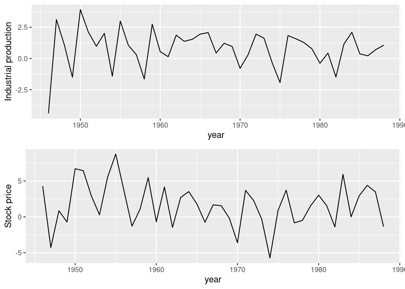
Figure 6.1: Time series of industrial production and stock prices in the NelPlo dataset.

The model will be fit using a single Gaussian likelihood so the data needs to be put as a single vector as well.

nelplo <- as.vector(NelPlo)

Next, the indices for the ar1 latent effect and the replicate effects are defined. This is done by taking the number of year first, n, and then creating the required indices. The index for the ar1 latent effect will go from 1 to \(n\) (and will be repeated once to cover both time series). The index for the replicate effect will go from 1 to 2, with the first \(n\) values having an index of 1 and the last \(n\) values of the data having an index of 2.

#Number of years
n <- nrow(NelPlo)

#Index for the ar1 latent effect
idx.ts <- rep(1:n, 2)

# Index for the replicate effect
idx.rep <- rep(1:2, each = n)

Two new variables are created to include two different intercepts for each part of the data:

# Intercepts
i1 <- c(rep(1, n), rep(NA, n))
i2 <- c(rep(NA, n), rep(1, n))

Finally, the model is fit as seen below. The fitted values are also computed (using the options in control.compute) and a vague prior on the precision of the random effects has been used (as described in Chapter 3).

m.rep <- inla(nelplo ~ -1 + i1 + i2 + 
  f(idx.ts, model = "ar1", replicate = idx.rep, 
    hyper = list(prec = list(param = c(0.001, 0.001)))),
  data = list(nelplo = nelplo, i1 = i1, i2 = i2, idx.ts = idx.ts,
    idx.rep = idx.rep),
  control.predictor = list(compute = TRUE)
)

summary(m.rep)

## 
## Call:
##    c("inla(formula = nelplo ~ -1 + i1 + i2 + f(idx.ts, model = 
##    \"ar1\", ", " replicate = idx.rep, hyper = list(prec = list(param 
##    = c(0.001, ", " 0.001)))), data = list(nelplo = nelplo, i1 = i1, 
##    i2 = i2, ", " idx.ts = idx.ts, idx.rep = idx.rep), 
##    control.predictor = list(compute = TRUE))" ) 
## Time used:
##     Pre = 0.229, Running = 0.248, Post = 0.0295, Total = 0.506 
## Fixed effects:
##     mean    sd 0.025quant 0.5quant 0.975quant  mode kld
## i1 0.790 0.369      0.064    0.790      1.516 0.790   0
## i2 1.674 0.369      0.948    1.674      2.399 1.674   0
## 
## Random effects:
##   Name     Model
##     idx.ts AR1 model
## 
## Model hyperparameters:
##                                           mean       sd 0.025quant
## Precision for the Gaussian observations  0.178 2.60e-02      0.131
## Precision for idx.ts                    68.816 3.41e+10      8.352
## Rho for idx.ts                           0.033 6.78e-01     -0.986
##                                         0.5quant 0.975quant   mode
## Precision for the Gaussian observations    0.176      0.233  0.174
## Precision for idx.ts                      56.624    195.185 28.259
## Rho for idx.ts                             0.087      0.976 -0.998
## 
## Expected number of effective parameters(stdev): 2.41(0.452)
## Number of equivalent replicates : 35.64 
## 
## Marginal log-Likelihood:  -223.14 
## Posterior marginals for the linear predictor and
##  the fitted values are computed

The model fit shows different estimates of the intercepts, which we had anticipated. However, the hyperparameters of the ar1 are shared between both time series.

Figure 6.2 shows the fitted values together with the observed values. It seems that the fitted values overfit the observed data, but see Chapter 8 and Chapter 9 for a discussion of these models and how to avoid overfitting. In general, overfitting can be avoided by setting specific priors on the model hyperparameters.

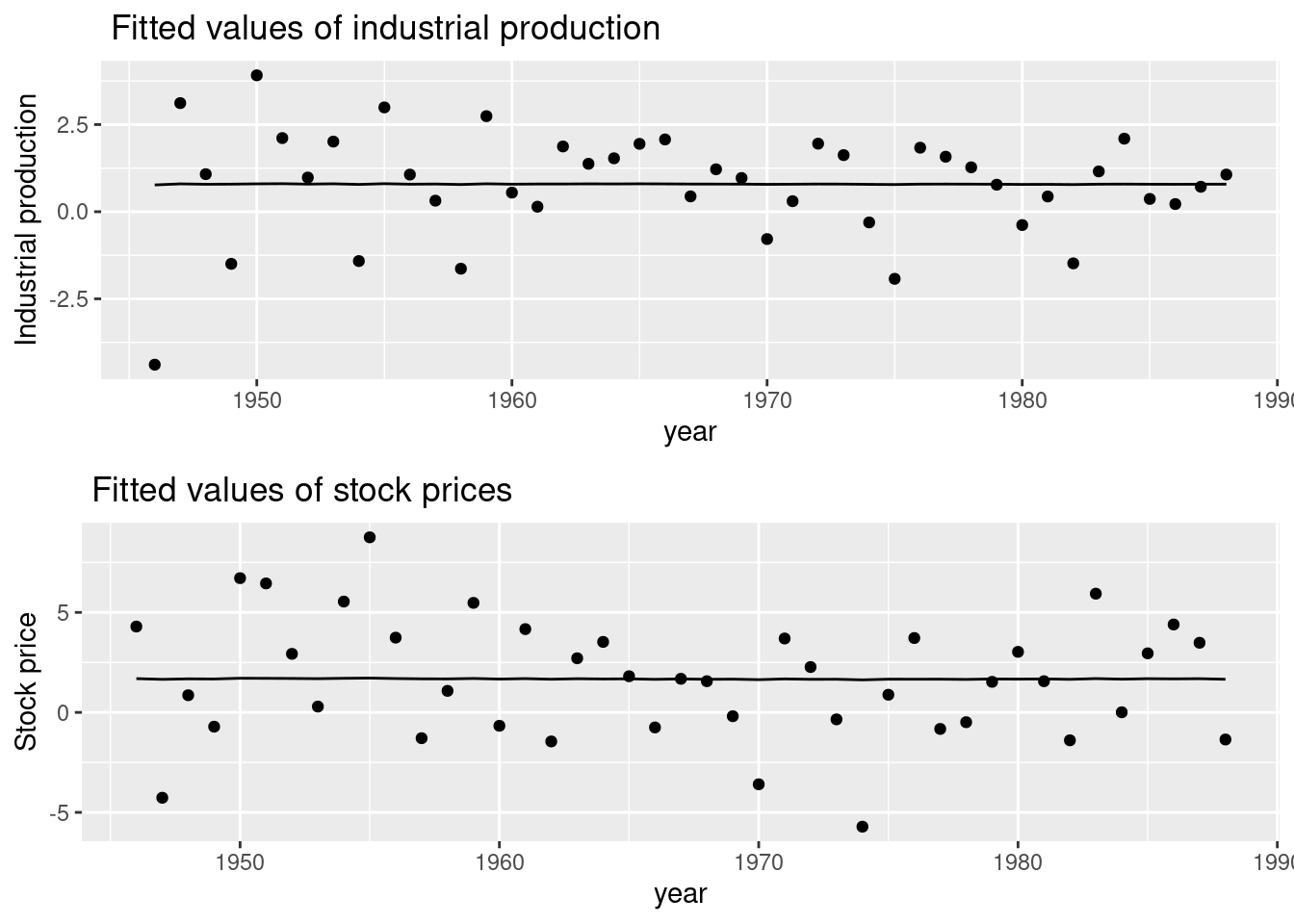
Figure 6.2: Fitted values (i.e., posterior means) to the variables in the NelPlo dataset using the replicate feature in INLA.

6.6 Linear constraints

As introduced in Chapter 3, additional linear constraints on the latent effects can be imposed. Given a latent effect \(\mathbf{u}\), the linear constraint is defined as

\[ \mathbf{A} \mathbf{u}^{\top} = \mathbf{e}^{\top} \]

where \(\mathbf{A}\) is a matrix with the same number of columns as the length of the latent effect \(\mathbf{u}\). Hence, the number of rows represents the number of linear constraints on the latent effect and \(\mathbf{e}\) is a vector of values that is defined accordingly.

Both \(\mathbf{A}\) and \(\mathbf{e}\) are passed through argument extraconstr using a named list with values A and e in the the definition of the latent effect using function f(). Note that there is another argument constr which can be used to add a sum-to-zero constraint on the latent effect by setting it to TRUE. This argument is set to TRUE for some latent effects (such as, for example, the rw1 and besag latent effects and other intrinsic effects). In case of doubt, the default option can be seen in the documentation available via the inla.doc() function.

Table 6.6: Arguments to be passed to the `f()` function to add constraints on the random effect.
Argument	Default	Description
`constr`	Depends on latent effect.	Add sum-to-zero constraint.
`extraconstr`	`list(A = NULL, e = NULL)`	Add extra constraints on the random effect.

Adding linear constraints is important in some cases as this makes the different effects in a model identifiable. Rue and Held (2005) describe this topic in detail. Furthermore, see Knorr-Held (2000) and Ugarte et al. (2014) on the role of imposing linear constraints to spatio-temporal latent effects, but these principles could also be applied to other types of latent effects. Also, Goicoa et al. (2018) note that adding additional constraints on the latent effects may produce different estimates than expected and caution should be taken when setting additional linear constraints.

As a simple example, we will add a sum to zero constraint to the ar1 model fit to the NelPLo dataset. In this case only the industrial production will be considered. We will also remove the intercept to show the effect of constraining the random effect.

First, the matrix A and vector e need to be defined:

# Define values of A and e to set linear constraints
A <- matrix(1, ncol = n, nrow = 1)
e <- matrix(0, ncol = 1)

Next, the model is fit using argument extraconstr in the call to the f() function that defines the latent effect. Remember that the intercept has the sole purpose of making the effect of the sum-to-zero constraint more evident.

m.unconstr <- inla(ip ~ -1 + f(idx, model = "ar1"),
  data = list(ip = NelPlo[, 1], idx = 1:n),
  control.family = list(hyper = list(prec = list(initial = 10,
    fixed = TRUE))),
  control.predictor = list(compute = TRUE)
)


m.constr <- inla(ip ~ -1 + f(idx, model = "ar1",
    extraconstr = list(A = A, e = e)),
  data = list(ip = NelPlo[, 1], idx = 1:n),
  control.family = list(hyper = list(prec = list(initial = 10,
    fixed = TRUE))),
  control.predictor = list(compute = TRUE)
)

Figure 6.3 shows the estimates of the random effects from both models. Note how now imposing the sum-to-zero constraint seems to provide slightly different estimates from the unconstrained estimates. It is possible that the estimates of other parameters in the model also change as a result of imposing a constraint on the random effects, as described in Goicoa et al. (2018).

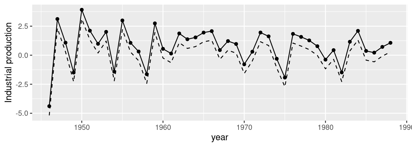
Figure 6.3: Comparison between two random effects estimates using a sum-to-zero constraint (solid line) and no constraint (dashed lines).

6.7 Final remarks

The features presented in this chapter can help to build more complex models using INLA. These are extensively used in some of the models used in other parts of the book. When the latent effect has a very complex structure that does not fit any of the latent effects described so far with the help of these additional features, there are a number of ways to implement custom latent effects for INLA. These methods are described in Chapter 11.

References

Bates, Douglas, and Martin Maechler. 2019. Matrix: Sparse and Dense Matrix Classes and Methods. https://CRAN.R-project.org/package=Matrix.

Davies, O. L. 1954. The Design and Analysis of Industrial Experiments. Wiley.

Faraway, J. 2006. Extending the Linear Model with R. Chapman; Hall, London.

Faraway, Julian. 2016. Faraway: Functions and Datasets for Books by Julian Faraway. https://CRAN.R-project.org/package=faraway.

Faraway, Julian J. 2019b. “INLA for Linear Mixed Models.” http://www.maths.bath.ac.uk/~jjf23/inla/.

Goicoa, T., A. Adin, M. D. Ugarte, and J. S. Hodges. 2018. “In Spatio-Temporal Disease Mapping Models, Identifiability Constraints Affect PQL and INLA Results.” Stochastic Environmental Research and Risk Assessment 3 (32): 749–70.

Knorr-Held, Leonhard. 2000. “Bayesian Modelling of Inseparable Space-Time Variation in Disease Risk.” Statistics in Medicine 19 (17‐18): 2555–67.

Koop, G., and M. F. J. Steel. 1994. “A Decision-Theoretic Analysis of the Unit-Root Hypothesis Using Mixtures of Elliptical Models.” Journal of Business and Economic Statistics 12: 95–107.

Krainski, Elias T., Virgilio Gómez-Rubio, Haakon Bakka, Amanda Lenzi, Daniela Castro-Camilo, Daniel Simpson, Finn Lindgren, and Håvard Rue. 2018. Advanced Spatial Modeling with Stochastic Partial Differential Equations Using R and INLA. Boca Raton, FL: Chapman & Hall/CRC.

Petris, Giovanni. 2010. “An R Package for Dynamic Linear Models.” Journal of Statistical Software 36 (12): 1–16. http://www.jstatsoft.org/v36/i12/.

Petris, Giovanni, Sonia Petrone, and Patrizia Campagnoli. 2009. Dynamic Linear Models with R. UseR! Springer-Verlag, New York.

Rue, H., and L. Held. 2005. Gaussian Markov Random Fields: Theory and Applications. Chapman; Hall/CRC Press.

Ugarte, M. D., A. Adin, T. Goicoa, and A. F. Militino. 2014. “On Fitting Spatio-Temporal Disease Mapping Models Using Approximate Bayesian Inference.” Statistical Methods in Medical Research 23: 507–30. https://doi.org/10.1177/0962280214527528.