Chapter 8 Temporal Models

8.1 Introduction

The analysis of time series refers to the analysis of data collected sequentially over time. Time can be indexed over a discrete domain (e.g., years) or a continuous one. In this section we will consider models to analyze both types of temporal data. The discrete case will be tackled with some of the autoregressive models covered in Chapter 3. The analysis of temporal data over a continuous domain will be done with smoothing methods described in Chapter 9. The analysis of space-time data will also be considered in the last part of this chapter. INLA provides a number of options to model data collected in space and time. Krainski et al. (2018) provides examples on space-time models for geostatistical data and point patterns, that we have omitted here.

This chapter starts with an introduction to the analysis of time series using autoregressive models in Section 8.2. Non-Gaussian time series are discussed in Section 8.3. Forecasting of time series is described in Section 8.4. Space-state models are in Section 8.5. Finally, Section 8.6 covers different types of space-time models.

8.2 Autoregressive models

When time is indexed over a discrete domain autoregressive models are a convenient way to model the data. Autoregressive models are described in Section 3.3 and in this chapter we will focus on providing some applications to temporal data.

As a first example of time series we will consider the climate reconstruction dataset analyzed in Fahrmeir and Kneib (2011). The original data is described in Moberg et al. (2005) and values represent the temperature anomalies (in Celsius degrees) from the Northern Hemisphere annual mean temperature 1961-90 average. Climate reconstruction is often based on indirect measurements from tree rings and other sources.

The variables in the dataset are available in Table 8.1. The original file has been obtained from the associated website of Fahrmeir and Kneib (2011). See Preface for details.

Table 8.1: Variables in the climate reconstruction dataset (Moberg et al. 2005; Fahrmeir and Kneib 2011).

Variable	Description
year	Year of measurement (from AD 1 to 1979).
temp	Temperature anomaly.

climate <- read.table(file = "data/moberg2005.raw.txt", header = TRUE)
summary(climate)

##       year           temp       
##  Min.   :   1   Min.   :-1.263  
##  1st Qu.: 496   1st Qu.:-0.489  
##  Median : 990   Median :-0.353  
##  Mean   : 990   Mean   :-0.354  
##  3rd Qu.:1484   3rd Qu.:-0.208  
##  Max.   :1979   Max.   : 0.372

Figure 8.1: Plot of the climate reconstrution dataset (Moberg et al. 2005, @FahrmeirKneib:2011).

The analysis will focus on estimating the main trend in the climate reconstruction time series. The model to be fit is an AR(1) on the year:

\[ y_t = \alpha + u_t + \varepsilon_t,\ t = 1, \ldots, 1979 \]

\[ u_1 \sim N(0, \tau_u (1-\rho^2)^{-1}) \]

\[ u_i = \rho u_{t-1} +\epsilon_t, \ t = 2, \ldots, 1979 \]

\[ \varepsilon_t \sim N(0, \tau_{\varepsilon}, t = 1, \ldots 1979 \]

Here, \(\alpha\) is an intercept, \(\rho\) a temporal correlation term (with \(|\rho| < 1\)) and \(\epsilon_t\) is a Gaussian error term with zero mean and precision \(\tau_u\). Note that variable \(y_t\) can be regarded as a Gaussian response with mean \(\alpha + u_t\) and a fixed large precision so that the error term is close to zero.

First of all, an AR(1) model will be fit:

climate.ar1 <- inla(temp ~ 1 + f(year, model = "ar1"), data = climate,
  control.predictor = list(compute = TRUE)
)
summary(climate.ar1)

## 
## Call:
##    c("inla(formula = temp ~ 1 + f(year, model = \"ar1\"), data = 
##    climate, ", " control.predictor = list(compute = TRUE))") 
## Time used:
##     Pre = 0.482, Running = 1.72, Post = 0.293, Total = 2.49 
## Fixed effects:
##               mean    sd 0.025quant 0.5quant 0.975quant   mode kld
## (Intercept) -0.352 0.023     -0.397   -0.352     -0.308 -0.353   0
## 
## Random effects:
##   Name     Model
##     year AR1 model
## 
## Model hyperparameters:
##                                             mean       sd 0.025quant
## Precision for the Gaussian observations 6.66e+04 2.29e+04   3.10e+04
## Precision for year                      2.07e+01 1.98e+00   1.72e+01
## Rho for year                            9.09e-01 9.00e-03   8.89e-01
##                                         0.5quant 0.975quant     mode
## Precision for the Gaussian observations 6.36e+04   1.22e+05 5.78e+04
## Precision for year                      2.06e+01   2.51e+01 2.02e+01
## Rho for year                            9.09e-01   9.24e-01 9.11e-01
## 
## Expected number of effective parameters(stdev): 1971.33(2.78)
## Number of equivalent replicates : 1.00 
## 
## Marginal log-Likelihood:  1896.03 
## Posterior marginals for the linear predictor and
##  the fitted values are computed

This model does not provide a good fit because it fits the observed data exactly, i.e., it overfits the data. For this reason, it is necessary to provide some prior information about what we expect the variation of the process to be. In the next example a prior Gamma with parameters 10 and 100 is used, so that the precision is centered at 0.1 and has a small variance of \(0.001\). Note that this prior is closer to the scale of the actual data than the default prior as the variance of temp is 0.0484. The prior is set by using the hyper argument inside the f() function where the ar1 latent effect is defined and in the control.family argument (for the precision of the likelihood).

climate.ar1 <- inla(temp ~ 1 + f(year, model = "ar1", 
    hyper = list(prec = list(param = c(10, 100)))), data = climate,
  control.predictor = list(compute = TRUE),
  control.compute = list(dic = TRUE, waic = TRUE, cpo = TRUE),
  control.family = list(hyper = list(prec = list(param = c(10, 100))))
)
summary(climate.ar1)

## 
## Call:
##    c("inla(formula = temp ~ 1 + f(year, model = \"ar1\", hyper = 
##    list(prec = list(param = c(10, ", " 100)))), data = climate, 
##    control.compute = list(dic = TRUE, ", " waic = TRUE, cpo = TRUE), 
##    control.predictor = list(compute = TRUE), ", " control.family = 
##    list(hyper = list(prec = list(param = c(10, ", " 100)))))") 
## Time used:
##     Pre = 0.224, Running = 2.76, Post = 0.141, Total = 3.12 
## Fixed effects:
##               mean    sd 0.025quant 0.5quant 0.975quant   mode kld
## (Intercept) -0.288 2.965     -6.161   -0.288      5.575 -0.288   0
## 
## Random effects:
##   Name     Model
##     year AR1 model
## 
## Model hyperparameters:
##                                          mean    sd 0.025quant 0.5quant
## Precision for the Gaussian observations 8.033 0.259      7.535    8.029
## Precision for year                      0.122 0.033      0.068    0.118
## Rho for year                            1.000 0.000      1.000    1.000
##                                         0.975quant  mode
## Precision for the Gaussian observations      8.555 8.022
## Precision for year                           0.199 0.111
## Rho for year                                 1.000 1.000
## 
## Expected number of effective parameters(stdev): 42.04(6.69)
## Number of equivalent replicates : 47.08 
## 
## Deviance Information Criterion (DIC) ...............: -50.99
## Deviance Information Criterion (DIC, saturated) ....: 434.63
## Effective number of parameters .....................: 42.51
## 
## Watanabe-Akaike information criterion (WAIC) ...: -84.97
## Effective number of parameters .................: 8.38
## 
## Marginal log-Likelihood:  -757.94 
## CPO and PIT are computed
## 
## Posterior marginals for the linear predictor and
##  the fitted values are computed

The next model to fit is a random walk of order 1:

\[ y_t = \alpha + u_t + \varepsilon_t,\ t = 1, \ldots 1979 \]

\[ u_t - u_{t-1} \sim N(0,\tau_u), \ t=2, \ldots, 1979 \]

\[ \varepsilon_t \sim N(0, \tau_{\varepsilon}), t = 1, \ldots 1979 \]

The model is fit similar to the ar1 models and we fix the precision of the Gaussian likelihood:

climate.rw1 <- inla(temp ~ 1 + f(year, model = "rw1", constr = FALSE,
    hyper = list(prec = list(param = c(10, 100)))), data = climate,
  control.predictor = list(compute = TRUE),
  control.compute = list(dic = TRUE, waic = TRUE, cpo = TRUE),
  control.family = list(hyper = list(prec = list(param = c(10, 100))))
)
summary(climate.rw1)

## 
## Call:
##    c("inla(formula = temp ~ 1 + f(year, model = \"rw1\", constr = 
##    FALSE, ", " hyper = list(prec = list(param = c(10, 100)))), data = 
##    climate, ", " control.compute = list(dic = TRUE, waic = TRUE, cpo 
##    = TRUE), ", " control.predictor = list(compute = TRUE), 
##    control.family = list(hyper = list(prec = list(param = c(10, ", " 
##    100)))))") 
## Time used:
##     Pre = 0.201, Running = 4.09, Post = 0.308, Total = 4.6 
## Fixed effects:
##              mean    sd 0.025quant 0.5quant 0.975quant  mode kld
## (Intercept) 0.003 603.3      -1258   -0.032       1258 0.001   0
## 
## Random effects:
##   Name     Model
##     year RW1 model
## 
## Model hyperparameters:
##                                         mean    sd 0.025quant 0.5quant
## Precision for the Gaussian observations 4.74 0.091       4.55     4.74
## Precision for year                      4.00 0.065       3.85     4.00
##                                         0.975quant mode
## Precision for the Gaussian observations       4.91 4.75
## Precision for year                            4.10 4.04
## 
## Expected number of effective parameters(stdev): 946.31(7.85)
## Number of equivalent replicates : 2.09 
## 
## Deviance Information Criterion (DIC) ...............: 2422.54
## Deviance Information Criterion (DIC, saturated) ....: 1872.36
## Effective number of parameters .....................: 928.67
## 
## Watanabe-Akaike information criterion (WAIC) ...: 1782.52
## Effective number of parameters .................: 233.11
## 
## Marginal log-Likelihood:  -2104.74 
## CPO and PIT are computed
## 
## Posterior marginals for the linear predictor and
##  the fitted values are computed

The model summary shows a strong temporal correlation, with a posterior mean of the parameter of 1.

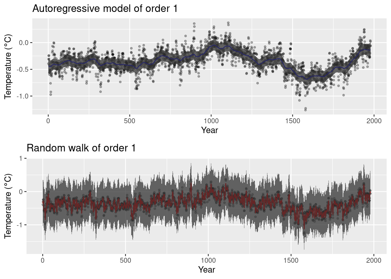
Figure 8.2: Models fit to the climate reconstruction dataset.

Figure 8.2 shows the posterior means and 95% credible intervals of the autoregressive and random walks models fit to the temperature data. The ar1 model produces smoother estimates than the rw1 model, which seems to overfit the data. Although both models use the same priors on the model precisions it is difficult to compare them directly unless the latent effects are scaled (see Section 5.6).

For both models the AIC and WAIC have been computed, and these clearly favor the ar1 model (probably because the rw1 overfits the data). Similarly, the CPO has been computed and they can be compared (see Section 2.4):

# ar1
- sum(log(climate.ar1$cpo$cpo))

## [1] -42.48

# rw1
- sum(log(climate.rw1$cpo$cpo))

## [1] 923.9

Again, this criterion shows a preference for the ar1 model.

8.3 Non-Gaussian data

Similar models can be fit to non-Gaussian data. The next example uses the number of yearly major earthquakes from 1900 to 2006 (Zucchini, MacDonald, and Langrock 2016). A major earthquake is one with a magnitude of 7 or greater. These are available in the earthquake dataset provided by the MixtureInf (Li, Chen, and Li 2016) package.

Table 8.2: Variables in the earthquake dataset.

Variable	Description
number	Number of major earthquakes (magnitude 7 or greater).

The earthquake data can be loaded and summarized as follows (norte that a new column with the year has been added as well):

library("MixtureInf")
data(earthquake)

#Add year
earthquake$year <- 1900:2006

#Summary of the data
summary(earthquake)

##      number          year     
##  Min.   : 6.0   Min.   :1900  
##  1st Qu.:15.0   1st Qu.:1926  
##  Median :18.0   Median :1953  
##  Mean   :19.4   Mean   :1953  
##  3rd Qu.:23.0   3rd Qu.:1980  
##  Max.   :41.0   Max.   :2006

Figure 8.3 shows the time series of the number of major earthquakes from 1900 to 2006.

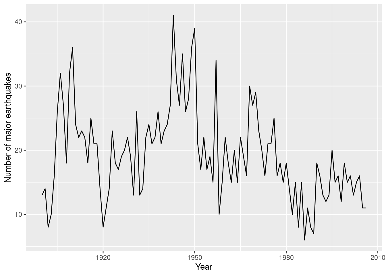
Figure 8.3: Number of major earthquakes from 1900 to 2006 in the earthquake dataset.

The first model to be fit to the earthquake data is an ar1:

\[ y_t \sim Po(\mu_t),\ t=1900, \ldots, 2006 \]

\[ \log(\mu_t) = \alpha + u_t,\ t=1900, \ldots, 2006 \]

\[ u_1 \sim N(0, \tau_u (1-\rho^2)^{-1}) \]

\[ u_i = \rho u_{t-1} +\epsilon_t, \ t = 2, \ldots, 1979 \]

\[ \epsilon_t \sim N(0, \tau_{\varepsilon}), \ t = 2, \ldots, 1979 \]

Note that now the distribution of the observed number of earthquakes is modeled using a Poisson distribution and that the linear predictor is linked to the mean using the natural logarithm.

quake.ar1 <- inla(number ~ 1 + f(year, model = "ar1"), data = earthquake,
  family = "poisson", control.predictor = list(compute = TRUE))
summary(quake.ar1)

## 
## Call:
##    c("inla(formula = number ~ 1 + f(year, model = \"ar1\"), family = 
##    \"poisson\", ", " data = earthquake, control.predictor = 
##    list(compute = TRUE))" ) 
## Time used:
##     Pre = 0.207, Running = 0.296, Post = 0.025, Total = 0.528 
## Fixed effects:
##              mean   sd 0.025quant 0.5quant 0.975quant  mode kld
## (Intercept) 2.863 0.19      2.436    2.877      3.191 2.891   0
## 
## Random effects:
##   Name     Model
##     year AR1 model
## 
## Model hyperparameters:
##                      mean   sd 0.025quant 0.5quant 0.975quant   mode
## Precision for year 12.055 4.67      4.870   11.449     22.951 10.116
## Rho for year        0.889 0.05      0.773    0.896      0.966  0.914
## 
## Expected number of effective parameters(stdev): 31.30(5.98)
## Number of equivalent replicates : 3.42 
## 
## Marginal log-Likelihood:  -343.45 
## Posterior marginals for the linear predictor and
##  the fitted values are computed

Similar to the climate example, a random walk of order one can be fit to the data:

\[ y_t \sim Po(\mu_t),\ t=1900, \ldots, 2006 \]

\[ \log(\mu_t) = \alpha + u_t \]

\[ u_t - u_{t-1} \sim N(0,\tau_u), \ t=2, \ldots, 1979 \]

This model is fit using the code below:

quake.rw1 <- inla(number ~ 1 + f(year, model = "rw1"), data = earthquake,
  family = "poisson", control.predictor = list(compute = TRUE))
summary(quake.rw1)

## 
## Call:
##    c("inla(formula = number ~ 1 + f(year, model = \"rw1\"), family = 
##    \"poisson\", ", " data = earthquake, control.predictor = 
##    list(compute = TRUE))" ) 
## Time used:
##     Pre = 0.202, Running = 0.132, Post = 0.026, Total = 0.361 
## Fixed effects:
##              mean    sd 0.025quant 0.5quant 0.975quant  mode kld
## (Intercept) 2.923 0.023      2.877    2.923      2.968 2.923   0
## 
## Random effects:
##   Name     Model
##     year RW1 model
## 
## Model hyperparameters:
##                     mean    sd 0.025quant 0.5quant 0.975quant  mode
## Precision for year 82.39 33.92      36.22    75.83     166.93 64.67
## 
## Expected number of effective parameters(stdev): 26.73(4.89)
## Number of equivalent replicates : 4.00 
## 
## Marginal log-Likelihood:  -342.67 
## Posterior marginals for the linear predictor and
##  the fitted values are computed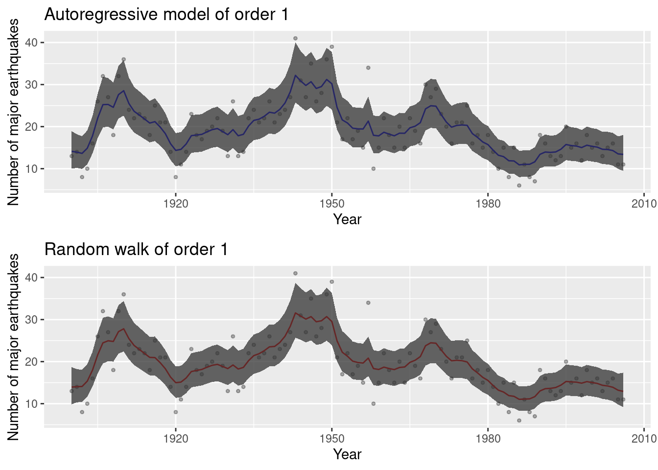

Figure 8.4: Models fit to the earthquake dataset.

Figure 8.4 shows the models fit to the earthquake dataset. This includes the posterior means and 95% credible intervals. Apparently, both models provide a similar fit to the data.

8.4 Forecasting

Time series forecasting in Bayesian inference can be regarded as fitting a model with some missing observations in the response, which requires computing the predictive distribution (see Section 12.3) at future times. If the model being fit includes covariates these must also be available as well for the years to be predicted. We will illustrate forecasting in time series with the earthquake dataset to try to estimate the future number of major earthquakes and the uncertainty about these estimates.

First of all, we use a few new lines (from year 2007 to 2020) to forecast the number of major earthquakes. These lines include the new time points (i.e., years) at which the prediction will be made and the number of earthquakes is set to NA for these new time points:

quake.pred <- rbind(earthquake, 
  data.frame(number = rep(NA, 14), year = 2007:2020))

Next, we fit the ar1 model to the new dataset so that the predictive distributions are computed:

quake.ar1.pred <- inla(number ~ 1 + f(year, model = "ar1"), data = quake.pred,
  family = "poisson", control.predictor = list(compute = TRUE, link = 1))
summary(quake.ar1.pred)

## 
## Call:
##    c("inla(formula = number ~ 1 + f(year, model = \"ar1\"), family = 
##    \"poisson\", ", " data = quake.pred, control.predictor = 
##    list(compute = TRUE, ", " link = 1))") 
## Time used:
##     Pre = 0.212, Running = 0.321, Post = 0.0253, Total = 0.559 
## Fixed effects:
##              mean   sd 0.025quant 0.5quant 0.975quant  mode kld
## (Intercept) 2.863 0.19      2.436    2.877      3.191 2.891   0
## 
## Random effects:
##   Name     Model
##     year AR1 model
## 
## Model hyperparameters:
##                      mean   sd 0.025quant 0.5quant 0.975quant   mode
## Precision for year 12.055 4.67      4.870   11.449     22.951 10.116
## Rho for year        0.889 0.05      0.773    0.896      0.966  0.914
## 
## Expected number of effective parameters(stdev): 31.30(5.98)
## Number of equivalent replicates : 3.42 
## 
## Marginal log-Likelihood:  -343.45 
## Posterior marginals for the linear predictor and
##  the fitted values are computed

In the previous code, the use of link = 1 is required so that predicted values are in the scale of the response, i.e., they are transformed taking the inverse of the link function. See 4.6 for details about the use of link in non-Gaussian models.

The mode fit is the same as the one obtained without the missing observations. Figure 8.5 shows the fitted and predicted values together with 95% credible intervals. Note how these get wider in the period from 2007 to 2020 as time progresses from the last year with observed data (i.e., 2006).

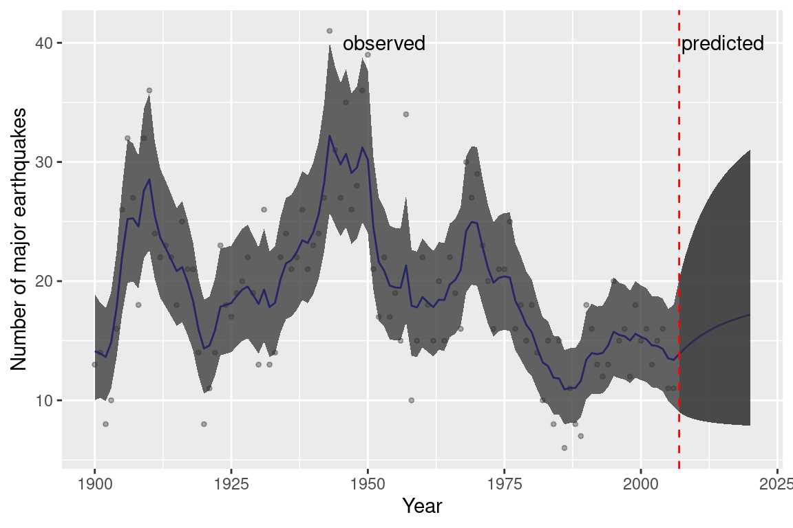
Figure 8.5: Prediction from the earthquake dataset from 2007 to 2020.

8.5 Space-state models

A class of temporal models where coefficients and other latent effects are allowed to change in time is that of dynamic models (Ruiz-Cárdenas, Krainski, and Rue 2012). These models can be summarized as follows:

\[ y_t = \beta_t x_t + \epsilon_t,\ \epsilon_t \sim N(0, \tau_t),\ t=1,\ldots, n \]

\[ x_t = \gamma_t x_{t-1} + \omega_t,\ \omega_t \sim N(0, \nu_t),\ t=2,\ldots, n \]

Here, \(y_t\) is a temporal observation, \(x_t\) is a state latent parameter, \(\beta_t\) and \(\gamma_t\) are temporally varying coefficients, and \(\epsilon_t\) and \(\omega_t\) are temporal errors or perturbations which follow a Gaussian distribution with 0 mean and precisions \(\tau_t\) and \(\nu_t\), respectively.

Latent effects \(\mathbf{x} = (x_1, \ldots, x_n))\) represent different states which need to be estimated. Note that they are not assigned a stochastic distribution because they are constants to be estimated. This will be simulated by modeling them using an iid distribution with a very large variance to conform to the unconstrained nature of these values.

Ruiz-Cárdenas, Krainski, and Rue (2012) describe how to use INLA to fit some classes of dynamic models when the data are fully observed. We will illustrate model fitting using a simple model.

\[ y_t = x_t + \nu_t,\ \nu_t \sim N(0, V),\ t=1,\ldots,n \]

\[ x_t = x_{t-1} + \omega_t,\ \omega_t \sim N(0,w),\ t = 2, \ldots, n \]

Note that in this case the temporal coefficients are constant and equal to one. Also, \((x_1,\ldots,x_n)\) is distributed as a random walk of order 1, which simplifies model fitting because the second equation above can be rewritten as:

\[ x_t - x_{t-1} = \omega_t,\ \omega_t \sim N(0,w),\ t = 2, \ldots, n \]

which is the definition of a first order random walk. Hence, model fitting here reduces to a model with a Gaussian response and random walk of order 1 in the linear predictor. However, we will describe the new approach developed in Ruiz-Cárdenas, Krainski, and Rue (2012) as this provides a more general framework to fit space-state models.

The second line in the previous equation can be rewritten as follows:

\[ 0 = x_t - x_{t-1} - \omega_t,\ \omega_t \sim N(0,w),\ t = 2, \ldots, n \]

This can be regarded as a submodel with “faked zero observations” which depends on the vector of latent effects \(\mathbf{x}\) and error terms \(\mathbf{\omega}\).

Hence, this model can be fit using two likelihoods (as explained in Section 6.4): one to fit the model that explains \(\mathbf{y}\) and the second one to fit the model that explains the “fake zero observations”. Given that both submodels depend on the same latent effects \(\mathbf{x}\), they can be shared between the two models using the copy feature described in Section 6.5.

8.5.1 Example: Alcohol consumption in Finland

As an example of the analysis of non-Gaussian data we will consider the analysis of alcohol related deaths in Finland in the period 1969-2013 in the age group between 30 and 39 years. This is available as dataset alcohol in package KFAS (Helske 2017), which is a time series object.

Table 8.3: Variables in the alcohol dataset.

Variable	Description
death at age 30-39	Number of alcohol related deaths (age group 30-39).
death at age 40-49	Number of alcohol related deaths (age group 40-49).
death at age 50-59	Number of alcohol related deaths (age group 50-59).
death at age 60-69	Number of alcohol related deaths (age group 60-69).
population by age 30-39	Population (age group 30-39) divided by 100000.
population by age 40-49	Population (age group 40-49) divided by 100000.
population by age 50-59	Population (age group 50-59) divided by 100000.
population by age 60-69	Population (age group 60-69) divided by 100000.

The alcohol dataset can be loaded with:

library("KFAS")
data(alcohol)

In order to fit a space-state model data need to be put in a two-column matrix as the model will contain two likelihoods, as explained in Section 6.4. In the first column, we will include the number of deaths in the age group 30-39, and in the second column the “fake zero” observations. Note that we have to remove the last row because it contains NA’s.

n <- nrow(alcohol) - 1 #There is an NA
Y <- matrix(NA, ncol = 2, nrow = n + (n - 1))
Y[1:n, 1] <- alcohol[1:n, 1]
Y[-c(1:n), 2] <- 0

The model will contain an offset with the population in the age group 30-39 for the data in the first column only:

#offset
oset <- c(alcohol[1:n, 5], rep(NA, n - 1))

Next, a number of indices and weights for the latent effect need to be created as well. These indices and weights are described in the formulation of the model above. Note that all indices have length \(n\) + \(n+1\) because the model will be made of two likelihoods. The first one is a Poisson likelihood to model the response, and the second one is a Gaussian likelihood to model the latent “fake zeroes” than define variable \(x_t\). When an index only works on one likelihood, then the corresponding values for the other likelihood will be set to NA.

#x_t
i <- c(1:n, 2:n)
#x_(t-1) 2:n
j <- c(rep(NA, n), 1:(n - 1))
# Weight to have -1 * x_(t-1)
w1 <- c(rep(NA, n), rep(-1, n - 1))
#x_(t-1), 2:n
l <- c(rep(NA, n), 2:n)
# Weight to have  * omega_(t-1)
w2 <- c(rep(NA, n), rep(-1, n - 1))

The final model is fit as follows:

prec.prior <- list(prec = list(param = c(0.001, 0.001)))
alc.inla <- inla(Y ~ 0 + offset(log(oset)) +
    f(i, model = "iid",
      hyper = list(prec = list(initial = -10, fixed = TRUE))) +
    f(j, w1, copy = "i") + f(l, w2, model = "iid"),
  data = list(Y = Y, oset = oset), family = c("poisson", "gaussian"),
  control.family = list(list(), 
    list(hyper = list(prec = list(initial = 10, fixed = TRUE)))),
  control.predictor = list(compute = TRUE)
)

Note that the previous model does not impose any distribution of the values of \(\mathbf{x}\) and they can take any values. For this reason, they have been included in the linear predictor using an iid model with a fixed tiny precision equal to \(\exp(-10)\), which is equivalent to having a large variance of \(\exp(10)\). That is, in practice effects in \(\mathbf{x}\) can take any value. Furthermore, control.family takes a list of two values (because of the two likelihoods) but only the second one is set because the first likelihoods do not require any extra constraints. The second argument is to fix the precision of the Gaussian likelihood.

The estimates and model fitting are summarized here:

summary(alc.inla)

## 
## Call:
##    c("inla(formula = Y ~ 0 + offset(log(oset)) + f(i, model = 
##    \"iid\", ", " hyper = list(prec = list(initial = -10, fixed = 
##    TRUE))) + ", " f(j, w1, copy = \"i\") + f(l, w2, model = \"iid\"), 
##    family = c(\"poisson\", ", " \"gaussian\"), data = list(Y = Y, 
##    oset = oset), control.predictor = list(compute = TRUE), ", " 
##    control.family = list(list(), list(hyper = list(prec = 
##    list(initial = 10, ", " fixed = TRUE)))))") 
## Time used:
##     Pre = 0.321, Running = 0.129, Post = 0.0246, Total = 0.475 
## Random effects:
##   Name     Model
##     i IID model
##    l IID model
##    j Copy
## 
## Model hyperparameters:
##                   mean    sd 0.025quant 0.5quant 0.975quant  mode
## Precision for l 111.08 53.31      43.38    99.63     245.91 81.26
## 
## Expected number of effective parameters(stdev): 63.52(3.50)
## Number of equivalent replicates : 1.37 
## 
## Marginal log-Likelihood:  -457.33 
## Posterior marginals for the linear predictor and
##  the fitted values are computed

Figure 8.6 shows the fitted values together with 95% credible intervals (shaded area). Note how the space-state model provides smoothed estimates.

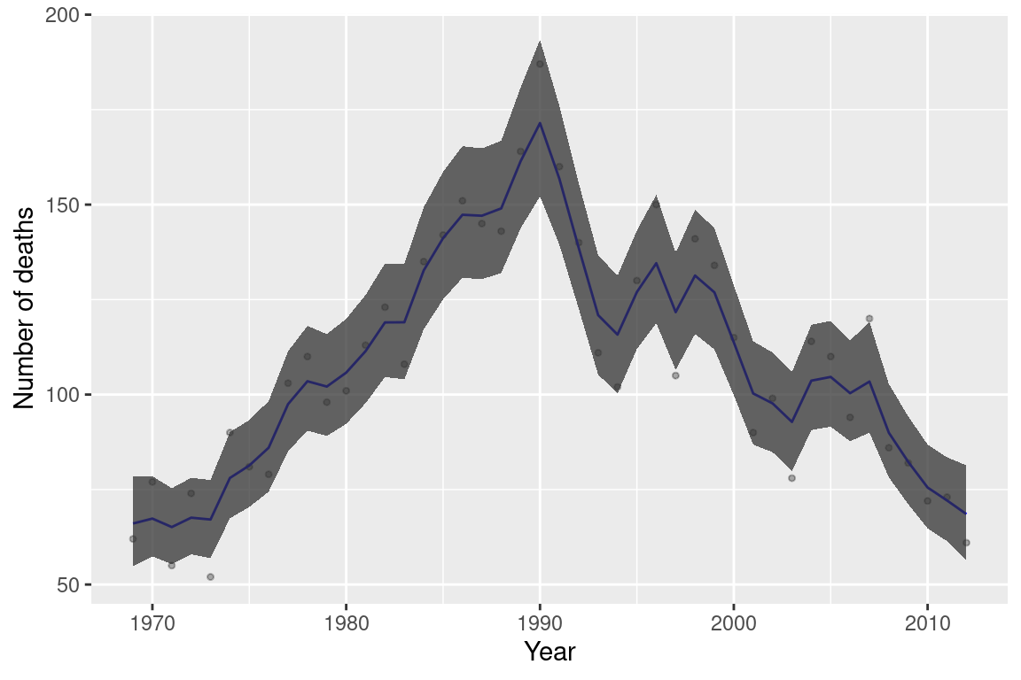
Figure 8.6: Space-state model fit to the alcohol dataset.

8.6 Spatio-temporal models

Spatial models have already been covered in Chapter 7. When time is also available, it is possible to build spatio-temporal models that include spatial and temporal random effects, as well as interaction effects between space and time.

A spatio-temporal model is said to be separable when the space-time covariance structure can be decomposed as a spatial and a temporal term. This often means that the spatio-temporal covariance can be written as a Kronecker product of a spatial and a temporal covariance (Fuentes, Chen, and Davis 2007) Non-separable covariance structures do not allow for a separate modeling of the spatial and temporal covariances (Wikle, Berliner, and Cressie 1998).

8.6.1 Separable models

Including separable spatial and temporal terms in the linear predictor can be done with ease by using the f() function to define two separate effects on space and time. Spatial effects are usually of the classes presented in Chapter 7, while temporal effects can be those presented in this chapter. However, latent effects used for spatial modeling can be used for temporal effects when the adjacency structure used reflects dependence between different temporal points.

The brainNM dataset from the DClusterm package (Gómez-Rubio, Moraga, et al. 2019) provides observed and expected counts of cases of brain cancer in the counties of New Mexico from 1973 to 1991 in a spatio-temporal STFDF object from the spacetime package (Pebesma 2012). The original data have been analyzed in Kulldorff et al. (1998). See the Preface for more information about the original data sources.

Table 8.4 shows the variables in the dataset, that can be loaded as follows:

library("DClusterm")
data(brainNM)

Table 8.4: Variables in the brainNM dataset.

Variable	Description
Observed	Observed number of cases.
Expected	Expected number of cases.
SMR	Standardized Mortality Ratio.
Year	Year.
FIPS	County FIPS code.
ID	County ID (from 1 to 32).
IDLANL	Inverse distance to Los Alamos National Laboratory.
IDLANLre	Re-scaled value of IDLANL by dividing by its mean.

A simple estimate of risk is the standardized mortality ratio (SMR) which is a simple estimate of the relative risk which is equal to the observed number of cases divided by the expected cases. Figure 8.7 shows the SMR for each county and year.

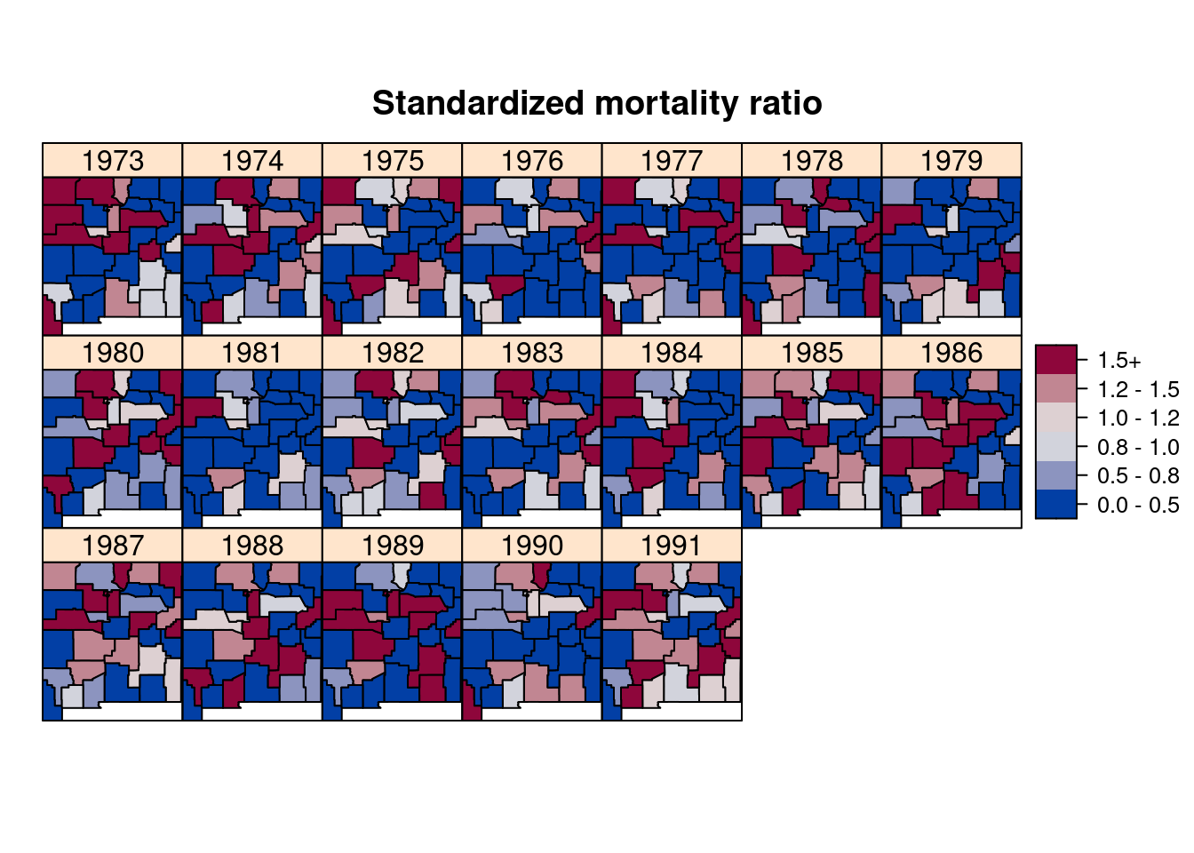
Figure 8.7: Standardized Mortality Ratio (SMR) of brain cancer in New Mexico from 1973 to 1991.

Before fitting the spatio-temporal model the adjacency structure of the counties in New Mexico is computed using function poly2nb() on the spatial object of the brainNM dataset.

nm.adj <- poly2nb(brainst@sp)
adj.mat <- as(nb2mat(nm.adj, style = "B"), "Matrix")

Next, the model is fit considering a separable model. In particular, the spatial effect is modeled using an ICAR model and the temporal trend using a rw1 latent effect. We will use vague priors (as in Chapter 3) to avoid overfitting.

# Prior of precision
prec.prior <- list(prec = list(param = c(0.001, 0.001)))

brain.st <- inla(Observed ~ 1 + f(Year, model = "rw1",
      hyper = prec.prior) + 
    f(as.numeric(ID), model = "besag", graph = adj.mat,
      hyper = prec.prior),
  data = brainst@data, E = Expected, family = "poisson",
  control.predictor = list(compute = TRUE, link = 1))
summary(brain.st)

## 
## Call:
##    c("inla(formula = Observed ~ 1 + f(Year, model = \"rw1\", hyper = 
##    prec.prior) + ", " f(as.numeric(ID), model = \"besag\", graph = 
##    adj.mat, hyper = prec.prior), ", " family = \"poisson\", data = 
##    brainst@data, E = Expected, control.predictor = list(compute = 
##    TRUE, ", " link = 1))") 
## Time used:
##     Pre = 0.305, Running = 0.557, Post = 0.0526, Total = 0.914 
## Fixed effects:
##               mean    sd 0.025quant 0.5quant 0.975quant   mode kld
## (Intercept) -0.048 0.038     -0.126   -0.047      0.025 -0.045   0
## 
## Random effects:
##   Name     Model
##     Year RW1 model
##    as.numeric(ID) Besags ICAR model
## 
## Model hyperparameters:
##                                mean     sd 0.025quant 0.5quant 0.975quant
## Precision for Year           484.88 525.71      55.10   328.80    1856.82
## Precision for as.numeric(ID)  65.37  88.71       7.51    39.03     285.08
##                                mode
## Precision for Year           145.71
## Precision for as.numeric(ID)  17.88
## 
## Expected number of effective parameters(stdev): 10.35(3.60)
## Number of equivalent replicates : 58.75 
## 
## Marginal log-Likelihood:  -824.58 
## Posterior marginals for the linear predictor and
##  the fitted values are computed

Figure 8.8 shows the estimated relative risk. Note how several counties in the center of the state show an increased risk throughout the whole period.

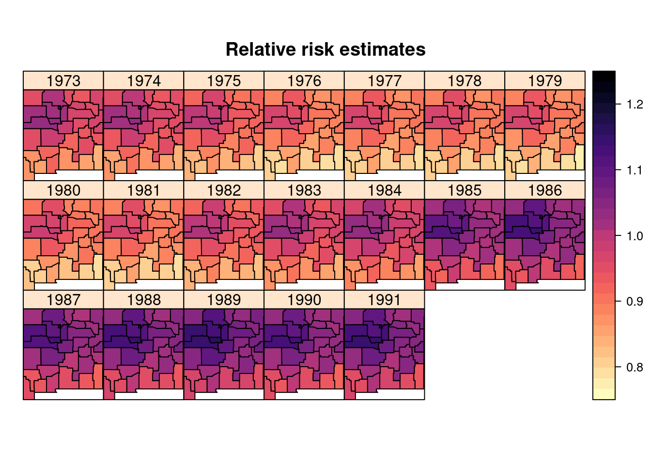
Figure 8.8: Posterior means of the relative risk estimate on the brainNM dataset.

This model assumes that the variation in each county is the sum of the spatial random effect and the overall temporal trend, i.e., there is no way to account for county-specific patterns. This may cause poor model fitting in some of the counties for certain years. Non-separable models may include space-time terms that account for this area-time interaction (Knorr-Held 2000).

8.6.2 Separable models with the group option

The f() function provides the group argument to set an index for the temporal structure of the data. This index will be used to define different types of temporal dependence, whose definition will be done via the control.group argument in the f() function.

Available models are

names(inla.models()$group)

## [1] "exchangeable"    "exchangeablepos" "ar1"             "ar"             
## [5] "rw1"             "rw2"             "besag"           "iid"

See Table 8.6 for a short summary of them. The options available to define the type of grouped effect and other required parameters is available in Table 8.5. Note that most of these options are only required if the latent effect defined in model needs them.

The resulting latent effect is a GMRF with zero mean and covariance matrix (Simpson 2016):

\[ \tau \Sigma_{b} \otimes \Sigma_{w} \]

where \(\Sigma_{b}\) is the structure of the covariance between the different groups and \(\Sigma_{w}\) the structure of the covariance matrix within each group.

The within-group effect is the one defined in the main f() function, while the between effect is the one defined using the control.group argument and it is of exchangeable type by default.

Table 8.5: Arguments available in control.group to define the temporal effect using the group argument.

Argument	Default	Description
model	"exchangeable"	Type of model.
order	NULL	Order of the model.
cyclic	FALSE	Whether this is a cyclic effect.
graph	NULL	Graph for spatial models.
scale.model	TRUE	Whether to scale the model.
adjust.for.con.comp	TRUE	Adjustment for non-connected components.
hyper	NULL	Definition of hyperprior.

Table 8.6: Types of latent effect in the group option.

Effect	Description
exchangeable	Exchangeable effect.
exchangeablepos	Exchangeable effect.
ar1	Autoregressive model of order 1.
ar	Autoregressive model of order \(p\).
rw1	Random walk of order 1.
rw2	Random walk of order 2.
besag	Besag spatial model.
iid	Independent and identically distributed random effects.

A similar model can be fit using the group argument. In this case, variable ID.Year is created to index the year (from 1 to 19) used to define the group. Argument control.group takes a list with the model (ar1) and other arguments to define this effect could be added. Index ID2 is created as a copy of the ID index so that it can be used in another latent effect.

brainst@data$ID.Year <- brainst@data$Year - 1973 + 1
brainst@data$ID2 <- brainst@data$ID

The model is then defined as in the code below. Note that the model includes only the spatio-temporal random effects. Note that this and the previous models are not exactly the same and that estimates may differ.

brain.st2 <- inla(Observed ~ 1 + 
    f(as.numeric(ID2), model = "besag", graph = adj.mat,
      group = ID.Year, control.group = list(model = "ar1"),
        hyper = prec.prior),
  data = brainst@data, E = Expected, family = "poisson",
  control.predictor = list(compute = TRUE, link = 1))
summary(brain.st2)

## 
## Call:
##    c("inla(formula = Observed ~ 1 + f(as.numeric(ID2), model = 
##    \"besag\", ", " graph = adj.mat, group = ID.Year, control.group = 
##    list(model = \"ar1\"), ", " hyper = prec.prior), family = 
##    \"poisson\", data = brainst@data, ", " E = Expected, 
##    control.predictor = list(compute = TRUE, link = 1))" ) 
## Time used:
##     Pre = 0.252, Running = 11.4, Post = 0.0526, Total = 11.7 
## Fixed effects:
##               mean    sd 0.025quant 0.5quant 0.975quant   mode kld
## (Intercept) -0.027 0.038     -0.105   -0.026      0.042 -0.022   0
## 
## Random effects:
##   Name     Model
##     as.numeric(ID2) Besags ICAR model
## 
## Model hyperparameters:
##                                 mean     sd 0.025quant 0.5quant 0.975quant
## Precision for as.numeric(ID2) 54.752 70.094       7.45   33.825    230.546
## GroupRho for as.numeric(ID2)   0.822  0.229       0.13    0.908      0.996
##                                 mode
## Precision for as.numeric(ID2) 16.814
## GroupRho for as.numeric(ID2)   0.992
## 
## Expected number of effective parameters(stdev): 9.40(7.14)
## Number of equivalent replicates : 64.64 
## 
## Marginal log-Likelihood:  -1196.66 
## Posterior marginals for the linear predictor and
##  the fitted values are computed

Figure 8.9 show the posterior means of the relative risk. Compared to the previous model this has a higher degree of smoothing. Note that this may be due to the fact that in the previous model the two effects were additive while now there is a single spatio-temporal effect. Furthermore, the estimate of the correlation of the ar1 model is large, which means that the model is assuming a high correlation (i.e., similarities) between consecutive years and very similar estimates from year to another are obtained.

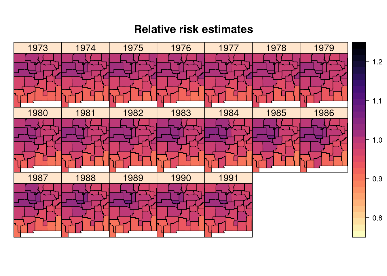
Figure 8.9: Posterior means of the relative risks obtained from a model using the group option fit to the brainNM dataset.

Non-separable models include an interaction term between space and time that cannot be decomposed as the product of two terms. These models can be fit with INLA but are harder to define. The specification of these models is not straightforward as it often requires imposing additional constraints on the space-time random effects (Knorr-Held 2000). Function inla.knmodels() can be used to fit these models with INLA. Goicoa et al. (2018) discuss the effect of imposing constraints on the space-time random effects and their impact on the estimates. Blangiardo and Cameletti (2015) cover some non-separable spatio-temporal models in Chapter 7.

8.7 Final remarks

Several types of spatial and spatio-temporal models that INLA can fit have been described in this chapter. Some of the latent effects mentioned here are also described in Chapter 3 and Chapter 9. For other models not implemented in INLA, the tools described in Chapter 11 can be used to implement new latent effects. Krainski et al. (2018) also propose a number of spatio-temporal models in the context of continuous processes and point processes.

Other spatio-temporal models that could be fit with INLA include those proposed in Knorr-Held (2000), which can be fit using function inla.knmodels(). Note that these models require imposing further constraints on the latent effects (see Section 6.6). Goicoa et al. (2018) discuss the effect of imposing constraints on the space-time random effects and their impact on the estimates.

Fitting non-separable spatio-temporal models with INLA is more difficult. Blangiardo and Cameletti (2015) cover some non-separable spatio-temporal models in Chapter 7. New models could be implemented using the methods described in Chapter 11 and, in particular, the rgeneric approach. Palmí-Perales, Gómez-Rubio, and Martínez-Beneito (2019) describe how to fit multivariate spatial latent effects with highly structured precision matrices that are implemented using rgeneric. This could be a guide on how to implement non-separable models because they often are based on specific parameterization of the spatio-temporal precision matrix.

References

Blangiardo, Marta, and Michela Cameletti. 2015. Spatial and Spatio-Temporal Bayesian Models with R-INLA. Chichester, UK: John Wiley & Sons Ltd.

Fahrmeir, Ludwig, and Thomas Kneib. 2011. Bayesian Smoothing Regression for Longitudinal, Spatial and Event History Data. New York: Oxford University Press.

Fuentes, M., L. Chen, and J. M. Davis. 2007. “A Class of Nonseparable and Nonstationary Spatial Temporal Covariance Functions.” Environmetrics 19 (5): 487–507. https://doi.org/doi:10.1002/env.891.

Goicoa, T., A. Adin, M. D. Ugarte, and J. S. Hodges. 2018. “In Spatio-Temporal Disease Mapping Models, Identifiability Constraints Affect PQL and INLA Results.” Stochastic Environmental Research and Risk Assessment 3 (32): 749–70.

Gómez-Rubio, Virgilio, Paula Moraga, John Molitor, and Barry Rowlingson. 2019. “DClusterm: Model-Based Detection of Disease Clusters.” Journal of Statistical Software, Articles 90 (14): 1–26. https://doi.org/10.18637/jss.v090.i14.

Helske, Jouni. 2017. “KFAS: Exponential Family State Space Models in R.” Journal of Statistical Software 78 (10): 1–39. https://doi.org/10.18637/jss.v078.i10.

Knorr-Held, Leonhard. 2000. “Bayesian Modelling of Inseparable Space-Time Variation in Disease Risk.” Statistics in Medicine 19 (17‐18): 2555–67.

Krainski, Elias T., Virgilio Gómez-Rubio, Haakon Bakka, Amanda Lenzi, Daniela Castro-Camilo, Daniel Simpson, Finn Lindgren, and Håvard Rue. 2018. Advanced Spatial Modeling with Stochastic Partial Differential Equations Using R and INLA. Boca Raton, FL: Chapman & Hall/CRC.

Kulldorff, M., W. F. Athas, E. J. Feurer, B. A. Miller, and C. R. Key. 1998. “Evaluating Cluster Alarms: A Space-Time Scan Statistic and Brain Cancer in Los Alamos, New Mexico.” American Journal of Public Health 88: 1377–80.

Li, Shaoting, Jiahua Chen, and Pengfei Li. 2016. MixtureInf: Inference for Finite Mixture Models. https://CRAN.R-project.org/package=MixtureInf.

Moberg, Anders, Dmitry M. Sonechkin, Karin Holmgren, Nina M. Datsenko, and Wibjörn Karlén. 2005. “Highly Variable Northern Hemisphere Temperatures Reconstructed from Low- and High-Resolution Proxy Data.” Nature 443: 613–17.

Palmí-Perales, Francisco, Virgilio Gómez-Rubio, and Miguel A. Martínez-Beneito. 2019. “Bayesian Multivariate Spatial Models for Lattice Data with INLA.” arXiv E-Prints, September, arXiv:1909.10804. http://arxiv.org/abs/1909.10804.

Pebesma, Edzer. 2012. “spacetime: Spatio-Temporal Data in R.” Journal of Statistical Software 51 (7): 1–30. http://www.jstatsoft.org/v51/i07/.

Ruiz-Cárdenas, R., E. T. Krainski, and H. Rue. 2012. “Direct Fitting of Dynamic Models Using Integrated Nested Laplace Approximations — INLA.” Computational Statistics & Data Analysis 56 (6): 1808–28. https://doi.org/http://dx.doi.org/10.1016/j.csda.2011.10.024.

Simpson, Daniel. 2016. “INLA for Spatial Statistics. Grouped Models.” http://faculty.washington.edu/jonno/SISMIDmaterial/8-Groupedmodels.pdf.

Wikle, C. K., L. M. Berliner, and N. Cressie. 1998. “Hierarchical Bayesian Space-Time Models.” Environmental and Ecological Statistics 5: 117–54.

Zucchini, W., I. L. MacDonald, and R. Langrock. 2016. Hidden Markov Models for Time Series: An Introduction Using R. 2nd ed. CRC Press.