Chapter 10 Survival Models

10.1 Introduction

Survival data analysis tackles the problem of modeling observations of time to event. In this context, the interest is the time until a certain event happens. This can be death (e.g., survival time since diagnosis) or failure (e.g., time until a piece breaks down). We will give a brief overview of survival analysis now, in order to introduce the main concepts and define our notation. A more comprehensive treatment of Bayesian survival analysis can be found in Ibrahim, Chen, and Sinha (2001). Moore (2016) also provides a nice introduction to survival analysis with R.

Considering T as the random variable that measures time to event, the survival function \(S(t)\) can be defined as the probability that \(T\) is higher than a given time \(t\), i.e., \(S(t) = P(T > t)\). For example, this could be the probability that a patient will survive at least until time \(t\) since diagnosis. In survival analysis there are the implicit assumptions that \(S(0) = 1\), i.e., all patients are alive at the beginning of the study, and that \(\lim_{t\to+\infty} S(t) = 0\), i.e., all patients will eventually die (Valar Morghullis).

When considering a survival function, it will be related to a distribution function \(F(t) = P(T <t) = 1 - S(t)\) with density function \(f(t)\). This can be a parametric distribution, as we will see below.

The hazard function \(h(t)\) measures the probability that the event occurs at a small instant given that the patient has survived until time \(t\). More precisely,

\[ h(t) = \lim_{\Delta t\to 0} \frac{P(T < t + \Delta t \mid T > t)}{\Delta t} \]

The cumulative hazard \(H(t)\) is defined as

\[ H(t) = \int_{0} ^t h(u) du \]

Hence, the hazard function can be expressed as \(h(t) = f(t) / S(t)\). Furthermore, the survival function can be expressed in terms of the cumulative hazard function as

\[ S(t) = \exp (-H(t)) \]

Survival data are often censored. For example, patients may experience the event during the study period, in which case the time to event is observed, or after the study has been finished, in which case the event time is unobserved. For this reason, each observation is accompanied by a status variable \(\delta_i\) to indicate whether the event was observed or not. In addition, a vector of covariates may be available for each patient. Hence, the data will be made of \(\{(t_i, \delta_i, \mathbf{x}_i\}_{i=1}^n\), where \(t_i\) is time of patient \(i\), \(\delta_i\) the associated censoring status variable and \(\mathbf{x}_i\) the covariates associated to patient \(i\).

The likelihood of this model can be expressed as:

\[ \prod_{i=1}^n f(t_i)^{\delta_i} S(t_i)^{1-\delta_i} \]

Note how depending on whether an observation has been censored its contribution to the likelihood will be either \(f(t_i)\) or \(S(t_i)\).

10.2 Non-parametric estimation of the survival curve

The Kaplan-Meier estimator provides a non-parametric estimate of the survival curve. It is based on the conditional probability of surviving until time \(t\) given that the patient has survived until time \(t_i\) and it is defined as

\[ \hat{S}(t) = \prod _{t_i \leq t} (1 - \frac{d_i}{n_i}) \]

Here, \(n_i\) is the number of subjects at risk at time \(i\) and \(d_i\) the number of individuals that fail at that time. Note that at a given time \(t_i\), \((1 - d_i/n_i)\) is the proportion of individuals at risk at time \(t_i\) that do not experience any event. Hence, the Kaplan-Meier estimate is the product of all conditional probabilities of not experiencing the event up to time \(t\).

The survival package (Terry M. Therneau and Patricia M. Grambsch 2000; Therneau 2015) implements a number of functions for the analysis of survival data, including the Kaplan-Meier estimator, and includes various datasets. We will be using the veteran dataset (Kalbfleisch and Prentice 1980), which contains data from the Veteran’s Administration Lung Cancer Trial. This dataset records time to death of 137 male patients with advanced inoperable lung cancer. Patients were assigned at random a standard treatment or a test treatment. Only 9 patients left the trial before they experienced death. In addition to the time to death and the treatment received, there are other covariates measured and they have been summarized in Table 10.1.

Table 10.1: Variables in the veteran dataset.

Variable	Description
trt	Treatment (1 for standard, 2 for test treatment)
celltype	Histological type of tumor (1=squamous, 2=smallcell, 3=adeno, 4=large).
time	Survival time (in days).
status	Censoring status (1 for death, 0 for censored).
karno	Karnofsky performance score (100 means good).
diagtime	Months from diagnosis to randomization.
age	Age in years.
prior	Prior therapy (0 for no, 10 for prior treatment).

First of all, we will load the data and recode some of the variables in the study as factors:

library("survival")
data(veteran) 

veteran$trt <- as.factor(veteran$trt)
levels(veteran$trt) <- c("standard", "test")
veteran$prior <- as.factor(veteran$prior)
levels(veteran$prior) <- c("No", "Yes")

As stated in the INLA documentation, some likelihoods for survival data may be affected by numerical overflow when observed times are large. For this reason, we will re-scale time before fitting any model and express time as 30-day months.

veteran$time.m <- round(veteran$time / 30, 3)

We will use the Surv() function to create a data structure with the required format for data analysis using the survival/censoring times and the censoring indicator. This is illustrated in the next lines where the first 20 values in the survival data structure are shown:

surv.vet <- Surv(veteran$time.m, veteran$status)
surv.vet[1:20]

##  [1]  2.400  13.700   7.600   4.200   3.933   0.333   2.733   3.667 
##  [9] 10.467   3.333+  1.400   0.267   4.800   0.833+  0.367   1.000 
## [17] 12.800   0.133   1.800   0.433

Note how censored observations are marked with a + to indicate that the time to event has been censored and it is larger than the value shown.

The Kaplan-Meier estimator can be used to obtain an estimate of the survival function as follows:

km.vet <- survfit(surv.vet ~ 1)

Figure 10.2 (left plot) shows a Kaplan-Meier estimate of the survival time for the veteran dataset. The plot includes confidence intervals as well as point estimates of the survival time. Note that the plot on the right corresponds to a parametric estimate discussed later in Section 10.3. They have been put side by side so that the different estimates can be compared.

Furthermore, four different survival curves can be estimated by splitting the data according to the different types of tumors:

km.vet.cell <- survfit(surv.vet ~ -1 + celltype, data = veteran)

Figure 10.1 shows estimates of the survival times for each of the four groups of patients defined by the covariate. Here, function autoplot() (in package ggpot2, Wickham 2016) has been used to produce the plot. Survival seems to be worst for those patients with tumors with a histological classification of adeno or smallcell.

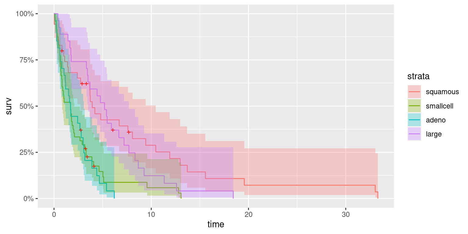
Figure 10.1: Survival estimates of patients according to histological type of tumor (i.e., cell type).

10.3 Parametric modeling of the survival function

INLA provides a number of distributions that can be used to model the survival function, as seen in Table 10.2.

For this first example we will fit a survival model to the the veteran dataset. INLA provides a similar function to Surv, called inla.surv, to create the necessary data structure to conduct a survival analysis, which is used as follows:

library("INLA")
sinla.vet <- inla.surv(veteran$time.m, veteran$status)

The model fitted to the veteran dataset in this first example is an exponential model. This corresponds to a model with constant hazard, i.e., \(h(t) = \lambda\), where \(\lambda\) is the rate parameter of the exponential distribution (see Table 10.2).

exp.vet <- inla(sinla.vet ~ 1, data = veteran, family = "exponential.surv")
summary(exp.vet)

## 
## Call:
##    "inla(formula = sinla.vet ~ 1, family = \"exponential.surv\", data 
##    = veteran)" 
## Time used:
##     Pre = 0.605, Running = 0.0532, Post = 0.0186, Total = 0.677 
## Fixed effects:
##               mean    sd 0.025quant 0.5quant 0.975quant   mode kld
## (Intercept) -1.468 0.088     -1.646   -1.466     -1.298 -1.463   0
## 
## Expected number of effective parameters(stdev): 1.00(0.00)
## Number of equivalent replicates : 136.89 
## 
## Marginal log-Likelihood:  -317.37

Table 10.2: Summary of some likelihoods available in INLA for survival analysis.

Likelihood	\(h(t)\)	\(H(t)\)	\(S(t)\)	family
Exponential	\(\lambda\)	\(\lambda t\)	\(\exp(-\lambda t)\)	exponential.surv
Weibull	\(\alpha \lambda(\lambda t)^{\alpha -1}\)	\((\lambda t)^{\alpha}\)	\(\exp(-(\lambda t)^{\alpha})\)	weibull.surv
Loglogistic	\(\frac{(\beta/\alpha)(t/\alpha)^{\beta-1}}{1+(t/\alpha)^{\beta}}\)	-	\((1+(t/\alpha)^{\beta})^{-1}\)	loglogistic.surv
Lognormal	-	-	-	lognormal.surv

In the previous model, a log link is used. Hence, \(\lambda = \exp(\alpha)\), where \(\alpha\) is the model intercept.

In this particular case, the survival function is

\[ S(t) = \exp(-H(t)) = \exp(-\int_0^t \lambda du) = \exp(-\lambda t) \]

We can use function inla.tmarginal() to transform the posterior marginal of \(\alpha\) into the marginal of \(S(t)\) for a given time and compute 95% credible intervals. Note that this is required because the intercept \(\alpha\) reported by INLA is actually \(\log(\lambda)\). Hence, for each time \(t\), the marginal of \(\alpha\) is transformed into the posterior marginal of \(S(t)\) and summary statistics are computed with function inla.zmarginal():

library("parallel")
# Set number of cores to use
options(mc.cores = 4)
# Grid of times
times <- seq(0.01, 35, by = 1)
# Marginal of alpha
alpha.marg <- exp.vet$marginals.fixed[["(Intercept)"]]
# Compute post. marg. of survival function
S.inla <- mclapply(times, function(t){
  S.marg <- inla.tmarginal(function(x) {exp(- exp(x) * t)}, alpha.marg)
  S.stats <- inla.zmarginal(S.marg, silent = TRUE)
  return(unlist(S.stats[c("quant0.025", "mean", "quant0.975")]))
})

S.inla <- as.data.frame(do.call(rbind, S.inla))

Figure 10.2 shows the survival function obtained with an exponential model. Median survival time is about 4 months, similar to the value obtained with the non-parametric Kaplan-Meier estimator. Furthermore, uncertainty is very similar between both estimates, with the credible intervals of the Bayesian parametric estimate narrower in the sides.

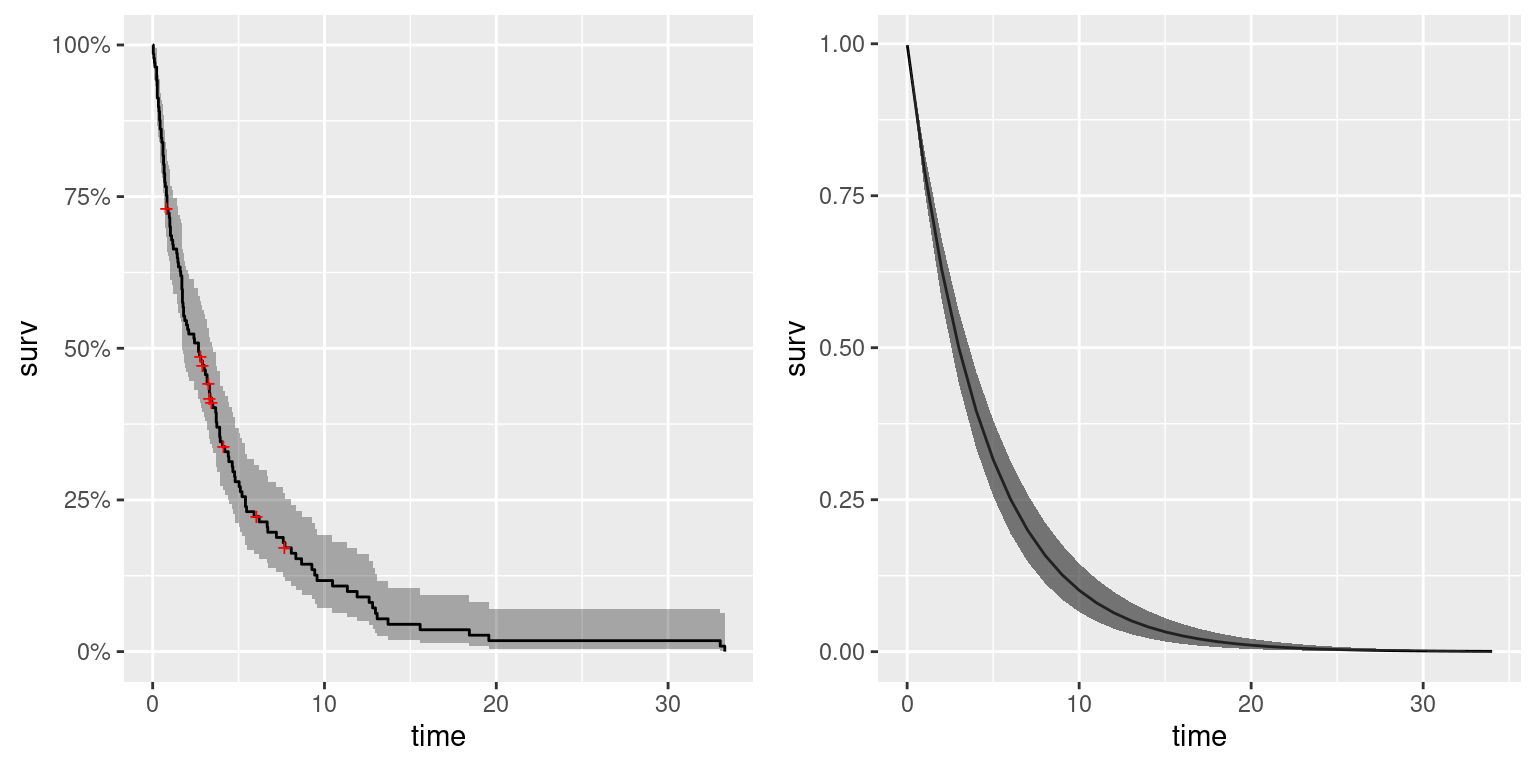
Figure 10.2: Kaplan-Meier estimate (left) and survival function using an exponential model (right) for the veteran dataset.

10.4 Semi-parametric estimation: Cox proportional hazards

Cox (1972) proposed a model in which the hazard function is the product of a baseline hazard \(h_0(t)\) and a term that depends on a number of covariates \(\mathbf{x}\). The baseline hazard can be estimated using non-parametric methods, while the term on the covariates is a function on a linear predictor on the covariates. In particular, a Cox proportional hazards models can be written down as:

\[ h(t) = h_0(t) \exp(\beta \mathbf{x}) \]

Hence, the hazard function is modulated by the covariates and their associated influence (as measured by coeffients \(\beta\)).

INLA implements a likelihood for a Cox proportional hazards model as follows:

\[ h(t) = h_0 (t) \exp(\eta) \]

Here, \(h_0(t)\) is the baseline hazard function and \(\eta\) is a linear predictor on some covariates and, possibly, other effects. Furthermore, the baseline hazard \(h_0(t)\) is modeled as:

\[ h_0(t) = \exp(b_k); t\in (s_{k-1}, s_{k}], k = 1, \ldots, K \]

Hence, the baseline hazard is a piecewise constant function. Variables \(\mathbf{b} = (b_1, \ldots, b_K)\) are assigned a prior which is a random walk of order 1 (default) or 2.

As described earlier, the veteran dataset includes a covariate that measures whether the patient received a standard treatment or a test treatment. We will use a Cox model to model survival time on this covariate and the type of tumor in order to assess the effect of the test treatment. Control option control.hazard (see Section 2.5) can be used to define a number of options on how the baseline hazard function is computed. Below, we only set the prior of the random effect to a vague prior (as seen in Chapter 3).

coxinla.vet <- inla(sinla.vet ~ 1  + celltype + trt, data = veteran,
  family = "coxph",
  control.hazard = list(hyper = list(prec = list(param = c(0.001, 0.001)))))
summary(coxinla.vet)

## 
## Call:
##    c("inla(formula = cph$formula, family = cph$family, contrasts = 
##    contrasts, ", " data = c(as.list(cph$data), cph$data.list), 
##    quantiles = quantiles, ", " E = cph$E, offset = offset, scale = 
##    scale, weights = weights, ", " Ntrials = NULL, strata = NULL, 
##    verbose = verbose, lincomb = lincomb, ", " selection = selection, 
##    control.compute = control.compute, ", " control.predictor = 
##    control.predictor, control.family = control.family, ", " 
##    control.inla = control.inla, control.results = control.results, ", 
##    " control.fixed = control.fixed, control.mode = control.mode, ", " 
##    control.expert = control.expert, control.hazard = control.hazard, 
##    ", " control.lincomb = control.lincomb, control.update = 
##    control.update, ", " control.pardiso = control.pardiso, 
##    only.hyperparam = only.hyperparam, ", " inla.call = inla.call, 
##    inla.arg = inla.arg, num.threads = num.threads, ", " 
##    blas.num.threads = blas.num.threads, keep = keep, 
##    working.directory = working.directory, ", " silent = silent, debug 
##    = debug)") 
## Time used:
##     Pre = 0.288, Running = 0.129, Post = 0.0229, Total = 0.44 
## Fixed effects:
##                     mean    sd 0.025quant 0.5quant 0.975quant   mode kld
## (Intercept)       -2.194 0.263     -2.731   -2.187     -1.698 -2.174   0
## celltypesmallcell  1.147 0.260      0.641    1.145      1.663  1.141   0
## celltypeadeno      1.216 0.279      0.664    1.217      1.761  1.220   0
## celltypelarge      0.324 0.280     -0.228    0.325      0.870  0.327   0
## trttest            0.169 0.194     -0.213    0.169      0.550  0.169   0
## 
## Random effects:
##   Name     Model
##     baseline.hazard RW1 model
## 
## Model hyperparameters:
##                                 mean     sd 0.025quant 0.5quant 0.975quant
## Precision for baseline.hazard 437.30 545.22      17.03   237.95    1977.19
##                                mode
## Precision for baseline.hazard 37.60
## 
## Expected number of effective parameters(stdev): 6.15(1.04)
## Number of equivalent replicates : 52.98 
## 
## Marginal log-Likelihood:  -365.47

The summary of the model indicates that survival depends on the type of tumor and that the test treatment does not seem to be better than the standard treatment.

The summary shows an estimate of the precision of the baseline hazard, which is modeled as a random walk of order 1 (in the log-scale). Because the estimate of the baseline risk is in the log-scale, we need to back-transform it and re-compute the summary statistics from the marginals:

#Transform baseline hazard
h0 <- lapply(coxinla.vet$marginals.random[["baseline.hazard"]],
  function(X) {inla.tmarginal(exp, X)}
)
#Compute summary statistics for plotting
h0.stats <- lapply(h0, inla.zmarginal)

Next, we have included the times and summary statistics of the baseline hazard together into a single data frame for plotting:

h0.df <- data.frame(t = coxinla.vet$summary.random[["baseline.hazard"]]$ID)
h0.df <- cbind(h0.df, do.call(rbind, lapply(h0.stats, unlist)))

Finally, Figure 10.3 shows the posterior means and 95% credible intervals of the baseline hazard function. We have added a red line to mark a hazard of 1. The estimated baseline hazard function seems to be constant about 1. This may occur because the covariates included in the model explain most of the variability in the data.

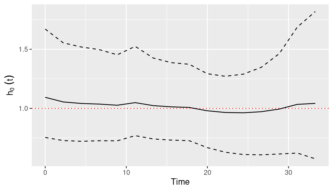
Figure 10.3: Posterior mean (solid line) and 95% credible interval (dashed lines) of baseline hazard function estimate using a Cox model on the veteran dataset.

10.5 Accelerated failure time models

Accelerated failure time (AFT) models are log-linear regression models that are widely applied in survival analysis. They take the following general form:

\[ \log(T) = \beta \mathbf{x} + \sigma \varepsilon \]

Here, \(\mathbf{x}\) is a vector of covariates with associated coefficients \(\beta\), \(\sigma\) is a precision parameter and \(\varepsilon\) is an error term. This error term can take different density distributions \(f_{\varepsilon}\) that will eventually define the survival and hazard functions.

Table 10.3: Summary of distributions used in accelerated time failure models.

Distribution of \(T\)	Distribution of error term (\(f_{\varepsilon}\))
Log-normal	Standard normal
Log-logistic	Logistic
Exponential	Extreme Value
Weibull	Extreme Value

Table 10.3 shows the distributions for the error term \(\varepsilon\) and the corresponding distribution of \(T\).

10.5.1 Log-normal model

The way to specify the AFT model to use with INLA is via the family option. In the next lines, a log-normal likelihood is used to fit a survival model to the veteran dataset:

logninla.vet <- inla(sinla.vet ~ -1 + celltype + trt, data = veteran,
  family = "lognormal.surv")

Note that the log-survival likelihood used in the model (i.e., lognormal.surv) is different from the typical log-normal distribution (i.e.,, lognormal), which does not takes censoring status into account.

The effects of the covariates on hazard can be assessed by checking the posterior summary statistics:

summary(logninla.vet)

## 
## Call:
##    c("inla(formula = sinla.vet ~ -1 + celltype + trt, family = 
##    \"lognormal.surv\", ", " data = veteran)") 
## Time used:
##     Pre = 0.204, Running = 0.071, Post = 0.0185, Total = 0.293 
## Fixed effects:
##                     mean    sd 0.025quant 0.5quant 0.975quant   mode kld
## celltypesquamous   1.254 0.266      0.734    1.254      1.779  1.252   0
## celltypesmallcell  0.420 0.211      0.005    0.419      0.835  0.419   0
## celltypeadeno      0.507 0.299     -0.080    0.506      1.094  0.506   0
## celltypelarge      1.495 0.276      0.953    1.495      2.038  1.494   0
## trttest           -0.214 0.234     -0.674   -0.214      0.245 -0.214   0
## 
## Model hyperparameters:
##                                               mean    sd 0.025quant
## Precision for the lognormalsurv observations 0.584 0.074      0.448
##                                              0.5quant 0.975quant  mode
## Precision for the lognormalsurv observations    0.581      0.738 0.574
## 
## Expected number of effective parameters(stdev): 5.00(0.00)
## Number of equivalent replicates : 27.40 
## 
## Marginal log-Likelihood:  -342.10

Given this model’s survival time, positive coefficients indicate a longer survival. For example, the effect of having an histological tumor of type large seems to provide the best survival among all patients.

In order to assess what risk factors increase survival time (and reduce hazard), the posterior probability of the coefficients of the fixed effects being positive can be computed with function inla.pmarginal():

lapply(logninla.vet$marginals.fixed, function(X){1 - inla.pmarginal(0, X)})

## $celltypesquamous
## [1] 1
## 
## $celltypesmallcell
## [1] 0.9764
## 
## $celltypeadeno
## [1] 0.955
## 
## $celltypelarge
## [1] 1
## 
## $trttest
## [1] 0.1779

Note that logninla.vet$marginals.fixed is a list with all the posterior marginals of the fixed effects. In order to compute the posterior probability of being lower than one, one minus the probability of being lower than zero is computed with 1 - inla.pmarginal(0, X) (where X represents a given posterior marginal).

10.5.2 Weibull model

Next, a Weibull survival model will be fitted to the veteran dataset:

weibinla.vet <- inla(sinla.vet ~ -1 + celltype + trt,
  data = veteran, family = "weibull.surv",
  control.family = list(variant=0))

The option control.family = list(variant=0) is used to use the following parameterisation for the distribution of time \(t\):

\[ f(t) = \alpha t^{\alpha - 1} \lambda \exp\{-\lambda t^{\alpha}\} \]

Then, the linear predictor \(\eta\) is linked to \(\lambda\) as \(\log(\lambda) = \eta\).

summary(weibinla.vet)

## 
## Call:
##    c("inla(formula = sinla.vet ~ -1 + celltype + trt, family = 
##    \"weibull.surv\", ", " data = veteran, control.family = 
##    list(variant = 0))") 
## Time used:
##     Pre = 0.202, Running = 0.101, Post = 0.0187, Total = 0.322 
## Fixed effects:
##                     mean    sd 0.025quant 0.5quant 0.975quant   mode kld
## celltypesquamous  -2.101 0.272     -2.648   -2.096     -1.581 -2.088   0
## celltypesmallcell -0.956 0.175     -1.309   -0.953     -0.623 -0.946   0
## celltypeadeno     -0.889 0.242     -1.382   -0.883     -0.431 -0.870   0
## celltypelarge     -1.777 0.236     -2.256   -1.771     -1.329 -1.761   0
## trttest            0.167 0.194     -0.214    0.167      0.547  0.167   0
## 
## Model hyperparameters:
##                                 mean    sd 0.025quant 0.5quant 0.975quant
## alpha parameter for weibullsurv 0.98 0.056      0.867    0.981       1.09
##                                  mode
## alpha parameter for weibullsurv 0.994
## 
## Expected number of effective parameters(stdev): 5.00(0.00)
## Number of equivalent replicates : 27.40 
## 
## Marginal log-Likelihood:  -322.59

Because of the parameterisation of this model, negative coefficients will increase survival time (and reduce hazard). Hence, the posterior probability of the coefficients being lower than zero can be computed to assess increased hazard:

lapply(weibinla.vet$marginals.fixed, function(X){inla.pmarginal(0, X)})

## $celltypesquamous
## [1] 1
## 
## $celltypesmallcell
## [1] 1
## 
## $celltypeadeno
## [1] 1
## 
## $celltypelarge
## [1] 1
## 
## $trttest
## [1] 0.1957

10.6 Frailty models

Under some circumstances, survival may be similar for certain patients. For example, members of a family may be resistant to certain types of cancer or pieces manufactured at a particular factory may have a lower quality that decreases survival time. This dependence means that observations are no longer independent within groups. This correlation is often modeled by means of random effects or frailties, in the survival argot.

Frailty models are essentially mixed-effects models for survival data. Sometimes survival data are clustered or grouped (i.e., families, schools, etc.) and observations are not independent. For this reason, random effects may be included in the survival model to account for correlation between subjects within groups. In the next examples we will show how to use INLA to fit these types of models.

The retinopathy dataset (Blair et al. 1976, @Husteretal:1989) in the survival package records data from a trial on laser coagulation treatment to delay diabetic retinopathy. This trial enrolled 197 patients with high-risk diabetic retinopathy and the event of interest was the time of loss of vision (measured as having a score below 5/200 in two consecutive visits). Each patient had one eye treated and the other eye was used as a control. Variables in this dataset are summarized in Table 10.4. In this case, between patient variation will be modeled using random effects in the frailty model.

Table 10.4: Variables in the retinopathy dataset.

Variable	Description
id	Patient identification number.
laser	Type of laser used (‘xenon’ or ‘argon’).
eye	Eye that was treated (‘right’ or ‘left’).
age	Age at the diagnosis of diabetes.
type	Type of diabetes (‘juvenile’ or ‘adult’).
trt	Treatment (0 for control eye, 1 for treated eye).
futime	Time to loss of vision or last follow-up (in months).
status	Censoring status (0 for censored, 1 for loss of vision).
risk	Risk score for the eye (values of 6 or greater indicate high risk).

First of all, the data will be loaded and the treatment variables converted into a factor:

data(retinopathy)

#Recode some covariates as factors
retinopathy$trt <- as.factor(c("control", "treated")[retinopathy$trt + 1])

#Summary
summary(retinopathy)

##        id         laser        eye           age             type    
##  Min.   :   5   xenon:200   right:178   Min.   : 1.0   juvenile:228  
##  1st Qu.: 480   argon:194   left :216   1st Qu.:10.0   adult   :166  
##  Median : 834                           Median :16.0                 
##  Mean   : 873                           Mean   :20.8                 
##  3rd Qu.:1296                           3rd Qu.:30.0                 
##  Max.   :1749                           Max.   :58.0                 
##       trt          futime         status           risk     
##  control:197   Min.   : 0.3   Min.   :0.000   Min.   : 6.0  
##  treated:197   1st Qu.:14.0   1st Qu.:0.000   1st Qu.: 9.0  
##                Median :38.8   Median :0.000   Median :10.0  
##                Mean   :35.6   Mean   :0.393   Mean   : 9.7  
##                3rd Qu.:54.2   3rd Qu.:1.000   3rd Qu.:11.0  
##                Max.   :75.0   Max.   :1.000   Max.   :12.0

In order to avoid numerical problems, the time to event has been converted into years:

retinopathy$futime <- retinopathy$futime / 12

A Kaplan-Meier estimate of the survival function can be obtained as:

surv.ret <- Surv(retinopathy$futime, retinopathy$status)

km.ret <- survfit(surv.ret ~ 1)

Figure 10.4 shows the Kaplan-Meier estimate. The large amount of censored observations above 70 months can be seen, which makes it difficult to estimate median survival time and survival for large periods of time.

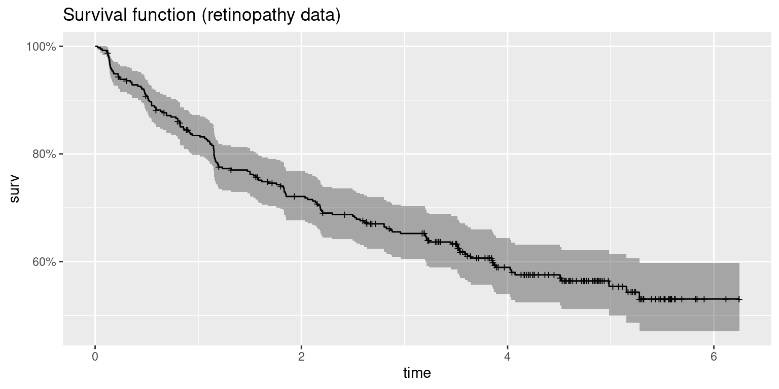
Figure 10.4: Survival function of the retinopathy dataset.

In this example we will consider a frailty model defined on patient (variable id) and a vague prior is used on the precision of the frailty effect:

# Model formula
form <- inla.surv(futime, status) ~ 1 + trt + risk + f(id, model = "iid",
  hyper = list(prec = list(param = c(0.001, 0.001))))

# Model fitting
fr.ret <- inla(form, data = retinopathy,
  family  = "weibullsurv")

Note that in the previous model the random effects are defined using a Gaussian distribution. A summary of the model is:

summary(fr.ret)

## 
## Call:
##    "inla(formula = form, family = \"weibullsurv\", data = 
##    retinopathy)" 
## Time used:
##     Pre = 0.227, Running = 0.45, Post = 0.0229, Total = 0.7 
## Fixed effects:
##               mean    sd 0.025quant 0.5quant 0.975quant   mode kld
## (Intercept) -3.369 0.704     -4.783   -3.358     -2.019 -3.335   0
## trttreated  -0.949 0.181     -1.310   -0.946     -0.599 -0.942   0
## risk         0.172 0.069      0.038    0.171      0.309  0.170   0
## 
## Random effects:
##   Name     Model
##     id IID model
## 
## Model hyperparameters:
##                                  mean    sd 0.025quant 0.5quant 0.975quant
## alpha parameter for weibullsurv 0.983 0.029      0.921    0.984       1.04
## Precision for id                1.204 0.491      0.585    1.090       2.46
##                                  mode
## alpha parameter for weibullsurv 0.991
## Precision for id                0.905
## 
## Expected number of effective parameters(stdev): 79.52(15.97)
## Number of equivalent replicates : 4.96 
## 
## Marginal log-Likelihood:  -457.95

The large precision of the frailties suggests that there is a small between patient variation given the other factors accounted for. Figure 10.5 shows 95% credible intervals of the frailties for each patient. These suggest that none of the patients have an intrinsic effect not accounted for by the covariates included in the model.

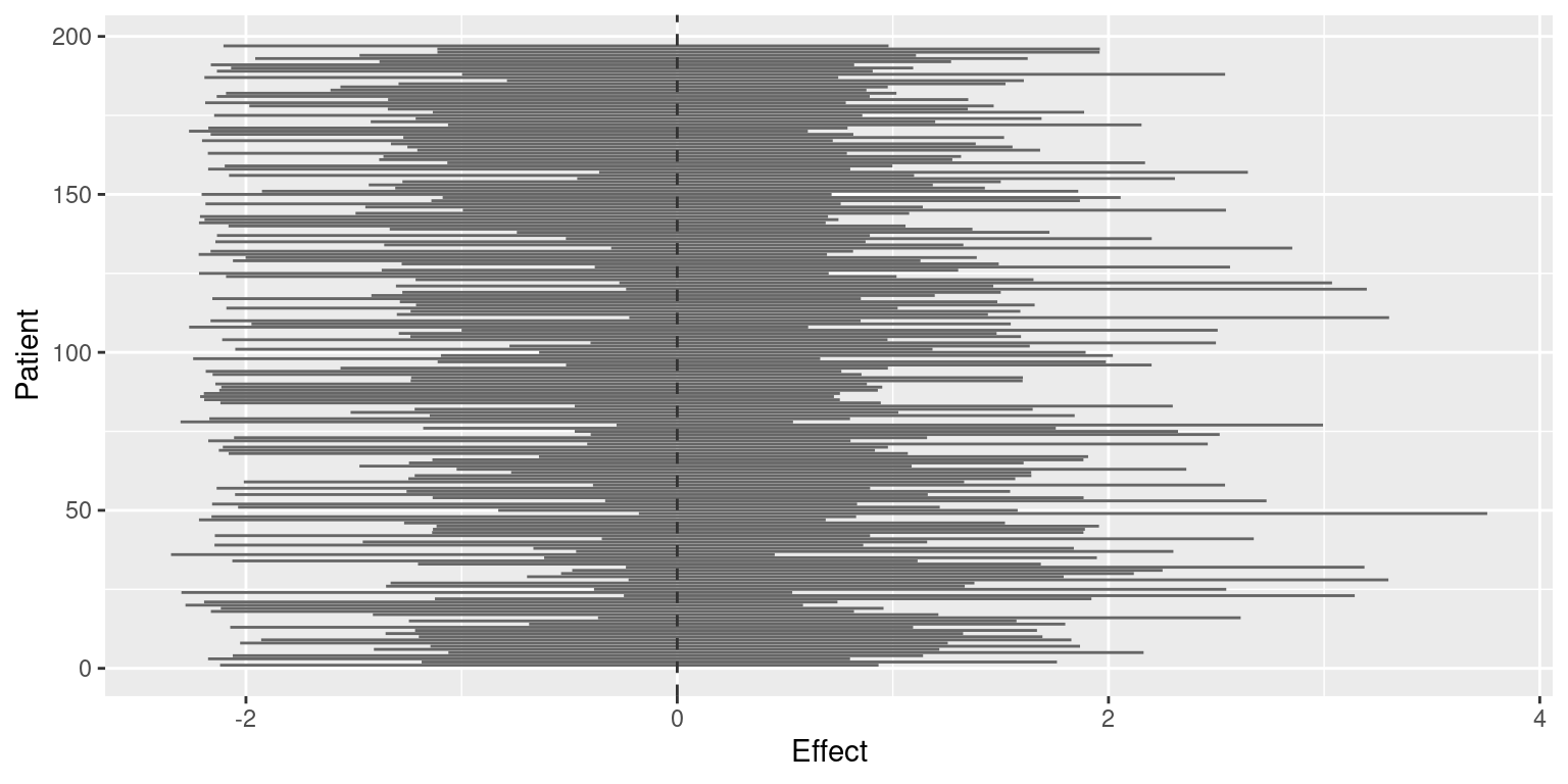
Figure 10.5: 95% credible intervals of the frailties in the retinopathy dataset analysis.

10.7 Joint modeling

So far, censorship and time to event have been assumed to be independent. However, these two variables may be correlated and relevant covariates may be available to explain this dependence. For example, patients may drop out from a clinical trial for a worsening in their clinical state. When clinical state can be modeled on several covariates using longitudinal data, censoring itself will also depend on these covariates. Hence, it is important to model clinical state (as measured by a convenient variable) and survival time.

This model will require a joint model with two components: a longitudinal model and a survival model. In practice, we will use a model with two likelihoods (see Section 6.4 for details) that share some latent effects. As an example, we will fit a joint model to a data set about 488 patients with liver cirrhosis in a randomized trial (Andersen et al. 1993). Prothrombin measurements were taken at irregular times as a measure of liver function. Furthermore, time to death (which can be censored) was also recorded for each patient. In addition, the randomized treatment for each patient (placebo or prednisone) is also available for all patients.

This dataset is available in package JMbayes (Rizopoulos 2016). The longitudinal and survival parts of the data set is available as prothro, while the survival part alone is prothros. In order to introduce the joint model step by step, we will fit a longitudinal model first, followed by a purely survival model and then the joint model.

10.7.1 Survival analysis

As stated before, the variables for the survival analysis are available in dataset prothros in package JMbayes. Table 10.5 shows a description of the variables in the dataset.

Table 10.5: Variables in the prothros dataset.

Variable	Description
id	Patient id number.
Time	Time to event or censoring time.
death	Indicator of whether the patient died (1) or not (0).
treat	Treatment (placebo or prednisone).

A summary of the variables in this dataset is shown below:

library("JMbayes")
data(prothros)
summary(prothros)

##        id           Time            death              treat    
##  Min.   :  1   Min.   : 0.011   Min.   :0.000   placebo   :251  
##  1st Qu.:167   1st Qu.: 0.632   1st Qu.:0.000   prednisone:237  
##  Median :302   Median : 2.616   Median :1.000                   
##  Mean   :295   Mean   : 3.643   Mean   :0.598                   
##  3rd Qu.:431   3rd Qu.: 6.236   3rd Qu.:1.000                   
##  Max.   :561   Max.   :13.394   Max.   :1.000

A survival model of the patients with treatment as a covariate can be fit to the data in order to assess the effect of the treatment and account for the variability between the patients. Note that for survival models time to event may be required to be re-scaled , e.g., to be in the \((0, 1)\) interval, to avoid numerical problems with INLA. In this case, no re-scaling is done.

#prothros$Time <- prothros$Time  / max(prothros$Time) # Re-scaling
pro.surv <- inla.surv(prothros$Time, prothros$death)

form.pro.surv <- pro.surv ~ 1 + treat

pro.surv.inla <- inla(form.pro.surv, data = prothros,
  family = "weibull.surv")

summary(pro.surv.inla)

## 
## Call:
##    "inla(formula = form.pro.surv, family = \"weibull.surv\", data = 
##    prothros)" 
## Time used:
##     Pre = 0.2, Running = 0.255, Post = 0.0167, Total = 0.472 
## Fixed effects:
##                   mean    sd 0.025quant 0.5quant 0.975quant   mode kld
## (Intercept)     -1.561 0.106     -1.774   -1.560     -1.357 -1.557   0
## treatprednisone  0.093 0.117     -0.137    0.093      0.323  0.093   0
## 
## Model hyperparameters:
##                                  mean   sd 0.025quant 0.5quant 0.975quant
## alpha parameter for weibullsurv 0.825 0.04      0.748    0.824      0.905
##                                  mode
## alpha parameter for weibullsurv 0.823
## 
## Expected number of effective parameters(stdev): 2.00(0.00)
## Number of equivalent replicates : 243.78 
## 
## Marginal log-Likelihood:  -815.53

The results show that prednisone has a positive coefficient but its effect does not seem to be significant, i.e., it does not increase survival time compared to the placebo.

10.7.2 Longitudinal analysis

Next, we will carry out a longitudinal analysis of the data to model how prothrombin measurements change over time. The longitudinal model will also consider the effect of treatment, which can be a placebo or prednisone.

Table 10.6: Variables in the prothro dataset.

Variable	Description
id	Patient id number.
pro	Prothrombin measurement.
time	Time of prothrombin measurement.
treat	Treatment (placebo or prednisone).
Time	Time to event or censoring time.
start	Time of prothrombin measurement.
stop	Time of next prothrombin measurement or to event or censoring time.
death	Indicator of whether the patient died (1) or not (0).
event	Indicator of whether the event was observed in this time interval (1) or not (0).

As stated earlier, the longitudinal data is available in dataset prothro in package JMbayes. Table 10.6 describes the variables in the longitudinal part of the dataset. Data is loaded and summarized below:

data(prothro)
summary(prothro)

##        id           pro           time               treat     
##  Min.   :  1   Min.   :  6   Min.   : 0.000   placebo   :1498  
##  1st Qu.:138   1st Qu.: 60   1st Qu.: 0.274   prednisone:1470  
##  Median :277   Median : 79   Median : 1.010                    
##  Mean   :277   Mean   : 79   Mean   : 2.039                    
##  3rd Qu.:418   3rd Qu.:100   3rd Qu.: 3.158                    
##  Max.   :561   Max.   :176   Max.   :11.108                    
##       Time            start             stop            death     
##  Min.   : 0.011   Min.   : 0.000   Min.   : 0.011   Min.   :0.00  
##  1st Qu.: 2.467   1st Qu.: 0.274   1st Qu.: 0.539   1st Qu.:0.00  
##  Median : 5.632   Median : 1.010   Median : 1.851   Median :1.00  
##  Mean   : 5.410   Mean   : 2.039   Mean   : 2.638   Mean   :0.55  
##  3rd Qu.: 8.145   3rd Qu.: 3.158   3rd Qu.: 4.082   3rd Qu.:1.00  
##  Max.   :13.394   Max.   :11.108   Max.   :13.394   Max.   :1.00  
##      event       
##  Min.   :0.0000  
##  1st Qu.:0.0000  
##  Median :0.0000  
##  Mean   :0.0984  
##  3rd Qu.:0.0000  
##  Max.   :1.0000

In this case, a longitudinal model is built to explain how prothrombin measurements change with time and according to treatment (as a fixed effect) or patient (included as a random effect). A log-normal likelihood is used in this case given that the response variable can only be positive:

form.pro.long <- pro ~ 1 + time + f(id, model = "iid") + treat
pro.long.inla <- inla(form.pro.long, data = prothro, family = "lognormal")
summary(pro.long.inla)

## 
## Call:
##    "inla(formula = form.pro.long, family = \"lognormal\", data = 
##    prothro)" 
## Time used:
##     Pre = 0.24, Running = 1.81, Post = 0.0375, Total = 2.08 
## Fixed effects:
##                   mean    sd 0.025quant 0.5quant 0.975quant   mode kld
## (Intercept)      4.264 0.021      4.223    4.264      4.306  4.264   0
## time             0.018 0.003      0.013    0.018      0.023  0.018   0
## treatprednisone -0.093 0.030     -0.151   -0.093     -0.034 -0.093   0
## 
## Random effects:
##   Name     Model
##     id IID model
## 
## Model hyperparameters:
##                                           mean    sd 0.025quant 0.5quant
## Precision for the lognormal observations 12.24 0.349      11.57    12.24
## Precision for id                         11.39 0.918       9.69    11.35
##                                          0.975quant  mode
## Precision for the lognormal observations      12.94 12.23
## Precision for id                              13.30 11.27
## 
## Expected number of effective parameters(stdev): 400.65(5.89)
## Number of equivalent replicates : 7.41 
## 
## Marginal log-Likelihood:  -13745.93

In this case, prothrombin increases with time but now patients treated with prednisone had lower values of prothrombin than patients treated with the placebo.

10.7.3 Joint model

For the joint model, we will be using a model with two likelihoods (see Section 6.4 for details), for the longitudinal and survival parts, respectively. First of all, we need to prepare the data. Using joint models with INLA is a bit tricky and requires extra preparation of the data.

First, we will create some auxiliary variables that we will use later. Essentially, these variables will help us fill the empty spaces of the variables used in the joint models with NA or zero.

#Number of observations in each dataset
n.l <- nrow(prothro)
n.s <- nrow(prothros)

#Vector of NA's
NAs.l <- rep(NA, n.l)
NAs.s <- rep(NA, n.s)
#Vector of zeros
zeros.l <- rep(0, n.l)
zeros.s <- rep(0, n.s)

The longitudinal and survival responses, now called Y.long and Y.surv, need to be expanded with NAs so that both variables have the same length and then put together in a list:

#Long. and survival responses
Y.long <- c(prothro$pro, NAs.s)
Y.surv <- inla.surv(time = c(NAs.l, prothros$Time),
  event = c(NAs.l, prothros$death))

Y.joint <- list(Y.long, Y.surv)

Covariates need to be expanded in a similar way:

#Covariates
covariates <- data.frame(
  #Intercepts (as factor with 2 levels)
  inter = as.factor(c(rep("b.l", n.l), rep("b.s", n.s))),
  #Time
  time.l = c(prothro$time, NAs.s),
  time.s = c(NAs.l, prothros$Time),
  #Treatment (longitudinal)
  treat.l = c(as.integer(prothro$treat =="prednisone"), NAs.s),
  #Treat.s
  treat.s = c(NAs.l, as.integer(prothros$treat =="prednisone"))
)

#Indices for random effects
r.effects <- list(
  #Patiend id (long.)
  id.l = c(prothro$id, NAs.s),
  #Patient id (surv.)
  id.s = c(NAs.l, prothros$id)
)

The last step in the data preparation step is to create a new object, joint.data, with the covariates, the indices of the random effects and the response variables:

joint.data  <- c(covariates, r.effects)
joint.data$Y <- Y.joint

10.7.4 Model with no shared terms

Once we have the data ready, we can proceed with model fitting. Firstly, we will fit a model with no shared terms between the longitudinal and the survival parts. Estimates from this model should match those obtained with the previous models:

pro.joint.inla <- inla(Y ~ -1 + inter +
    # Longitudinal part
    f(id.l) + 
    time.l + treat.l +
    #Survival part
    treat.s,
  data = joint.data, family = c("lognormal", "weibull.surv")
)

summary(pro.joint.inla)

## 
## Call:
##    c("inla(formula = Y ~ -1 + inter + f(id.l) + time.l + treat.l + ", 
##    " treat.s, family = c(\"lognormal\", \"weibull.surv\"), data = 
##    joint.data)" ) 
## Time used:
##     Pre = 0.286, Running = 1.93, Post = 0.0358, Total = 2.26 
## Fixed effects:
##            mean    sd 0.025quant 0.5quant 0.975quant   mode kld
## interb.l  4.264 0.021      4.223    4.264      4.306  4.264   0
## interb.s -1.563 0.106     -1.773   -1.562     -1.359 -1.560   0
## time.l    0.018 0.003      0.013    0.018      0.023  0.018   0
## treat.l  -0.093 0.030     -0.151   -0.093     -0.034 -0.093   0
## treat.s   0.093 0.117     -0.137    0.093      0.323  0.093   0
## 
## Random effects:
##   Name     Model
##     id.l IID model
## 
## Model hyperparameters:
##                                            mean    sd 0.025quant 0.5quant
## Precision for the lognormal observations 12.244 0.350     11.568   12.240
## alpha parameter for weibullsurv[2]        0.825 0.040      0.749    0.824
## Precision for id.l                       11.392 0.922      9.682   11.357
##                                          0.975quant   mode
## Precision for the lognormal observations     12.945 12.233
## alpha parameter for weibullsurv[2]            0.904  0.824
## Precision for id.l                           13.309 11.289
## 
## Expected number of effective parameters(stdev): 402.64(5.78)
## Number of equivalent replicates : 8.58 
## 
## Marginal log-Likelihood:  -14570.69

Note how the point estimates of this model are very close to the one obtained for the independent survival and longitudinal models fit earlier in this section.

10.7.5 Joint model with correlated terms

Next, we will fit a joint model where some effects are shared between both parts of the model. In particular, a patient specific intercept and coefficient on time is considered in the longitudinal model with a different intercept and coefficient per patient, and these are copied into the survival model multiplied by a scaling coefficient (which is the same for all patients, but different from the intercepts and coefficient on time).

The longitudinal model that we are trying to fit includes fixed effects on time of measurement (time) and treatment (trt), a random intercept and random coefficient on time for each patient:

\[ y_j \sim lognorm(\mu_j, \tau),\ j = 1,\ldots, 2968 \]

\[ \mu_j = \beta_{l,0} + \beta_{l, t} \cdot t_j + \beta_{l, trt} \cdot trt_j + \beta_{1, i(j)} + \beta_{2, i(j)} t_j \]

Note that index \(j\) indicates the row of the table in the prothros dataset (which included repeated observations per patient) and that index \(i(j)\) is used to identify the patient to which data in row \(j\) belongs.

Similarly, the survival part of the model contains a fixed effect on treatment plus copied effects of the random intercept and coefficient:

\[ t_i \sim Weib(\lambda_i, \alpha),\ i = 1,\ldots, 488 \]

\[ \log(\lambda_i) = \beta_{s,0} + \beta_{s,trt} \cdot trt_i + \beta_1 \cdot \beta_{1, i} + \beta_2 \cdot \beta_{2, i} \cdot t_i \]

This model requires a bit of data preparation before it can be fit. First of all, unique ids of the patients are obtained to be used in both parts of the model. This is done by collecting the list of unique ids and matching variable id in the longitudinal and survival datasets:

#Unique index for patient from 1 to n.patients
unique.id <- unique(prothro$id)
n.id <- length(unique.id)
idx <- 1:n.id

#Unique indices for long. and survival data
idx.l <- match(prothro$id, unique.id )
idx.s <- match(prothros$id, unique.id )

Then, indices are created to indicate the patients in the longitudinal and survival part of the model:

#Indices for random intercept
joint.data$idx.sh.l <- c(idx.l, NAs.s)
joint.data$idx.sh.l2 <- c(idx.l, NAs.s)

#Indices for coefficient of time
joint.data$idx.sh.s <- c(NAs.l, idx.s)
joint.data$idx.sh.s2 <- c(NAs.l, idx.s)

Note that these indices will be used to identify (using the patient’s id) the random intercept and coefficient of time in order to be able to copy the effects of \(\beta_{1,i}\) and \(\beta_{2,i}\). Given that we are copying two effects, two sets of indices are required.

Now, we can display the estimates of the shared random effects that have been ‘copied’ from the longitudinal part of the model to the survival part. Shared components are defined in INLA using the copy feature:

pro.joint.inla2 <- inla(Y ~ -1 +
    #Intercepts
    inter +
    #Longitudinal model
    time.l + treat.l +
    f(idx.sh.l, model = "iid") +
    f(idx.sh.l2, time.l, model = "iid") +
    #Survival model
    treat.s +
    f(idx.sh.s, copy = "idx.sh.l", fixed = FALSE) +
    f(idx.sh.s2, time.s, copy = "idx.sh.l", fixed = FALSE),
  data = joint.data,
  family = c("lognormal", "weibull.surv")
)

summary(pro.joint.inla2)

## 
## Call:
##    c("inla(formula = Y ~ -1 + inter + time.l + treat.l + f(idx.sh.l, 
##    ", " model = \"iid\") + f(idx.sh.l2, time.l, model = \"iid\") + 
##    treat.s + ", " f(idx.sh.s, copy = \"idx.sh.l\", fixed = FALSE) + 
##    f(idx.sh.s2, ", " time.s, copy = \"idx.sh.l\", fixed = FALSE), 
##    family = c(\"lognormal\", ", " \"weibull.surv\"), data = 
##    joint.data)") 
## Time used:
##     Pre = 0.48, Running = 12.7, Post = 0.0787, Total = 13.2 
## Fixed effects:
##            mean    sd 0.025quant 0.5quant 0.975quant   mode kld
## interb.l  4.238 0.025      4.189    4.238      4.286  4.237   0
## interb.s -1.493 0.115     -1.720   -1.492     -1.269 -1.491   0
## time.l    0.007 0.005     -0.003    0.007      0.016  0.007   0
## treat.l  -0.100 0.030     -0.159   -0.100     -0.040 -0.100   0
## treat.s   0.082 0.127     -0.167    0.082      0.331  0.082   0
## 
## Random effects:
##   Name     Model
##     idx.sh.l IID model
##    idx.sh.l2 IID model
##    idx.sh.s Copy
##    idx.sh.s2 Copy
## 
## Model hyperparameters:
##                                             mean     sd 0.025quant
## Precision for the lognormal observations  14.203  0.456     13.310
## alpha parameter for weibullsurv[2]         0.867  0.045      0.775
## Precision for idx.sh.l                    11.005  1.007      9.313
## Precision for idx.sh.l2                  314.121 68.513    202.719
## Beta for idx.sh.s                         -0.445  0.323     -1.092
## Beta for idx.sh.s2                        -0.191  0.073     -0.335
##                                          0.5quant 0.975quant    mode
## Precision for the lognormal observations   14.204     15.101  14.217
## alpha parameter for weibullsurv[2]          0.870      0.949   0.880
## Precision for idx.sh.l                     10.897     13.247  10.609
## Precision for idx.sh.l2                   306.099    470.172 290.402
## Beta for idx.sh.s                          -0.440      0.180  -0.422
## Beta for idx.sh.s2                         -0.192     -0.047  -0.192
## 
## Expected number of effective parameters(stdev): 554.73(13.60)
## Number of equivalent replicates : 6.23 
## 
## Marginal log-Likelihood:  -14513.11

The effect on the copied effects is measured by hyperparameters Beta. Beta for idx.sh.s is the one that multiplies the patient specific intercept in the longitudinal model to add it to the linear predictor of the survival model, while Beta for idx.sh.s2 is the one that multiplies the shared effect on time.

Figure 10.6 displays the patient specific intercepts and their respective copied values into the survival model. There is a linear dependence between them because the random effects in the survival part are the random effects in the longitudinal part multiplied by a constant scaling factor. The red line is a line with slope the posterior mean of the scaling factor.

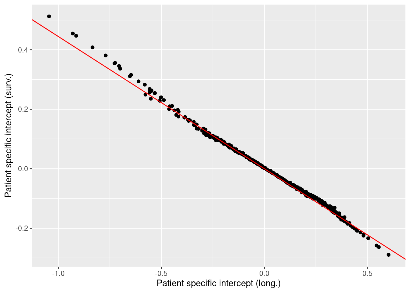
Figure 10.6: Patient specific intercept in the longitudinal models versus their copied values into the survival model. The red line represents a line with slope equal to the posterior mean of the scaling factor \(\beta_1\).

References

Andersen, P. K., O. Borgan, R. D. Gill, and N. Keiding. 1993. Statistical Models Based on Counting Processes. New York: Springer.

Blair, A. L., D. R. Hadden, J. A. Weaver, D. B. Archer, P. B. Johnston, and C. J. Maguire. 1976. “The 5-Year Prognosis for Vision in Diabetes.” American Journal of Ophthalmology 81: 383–96.

Cox, D. R. 1972. “Regression Models and Life-Tables.” Journal of the Royal Statistical Society. Series B 34 (2): 187–220.

Ibrahim, Joseph G., Ming-Hui Chen, and Debajyoti Sinha. 2001. Bayesian Survival Analysis. Springer.

Kalbfleisch, D., and R. L. Prentice. 1980. The Statistical Analysis of Failure Time Data. New York: Wiley.

Moore, Dirk F. 2016. Applied Survival Analysis Using R. Springer.

Rizopoulos, Dimitris. 2016. “The R Package JMbayes for Fitting Joint Models for Longitudinal and Time-to-Event Data Using Mcmc.” Journal of Statistical Software 72 (7): 1–45. https://doi.org/10.18637/jss.v072.i07.

Terry M. Therneau, and Patricia M. Grambsch. 2000. Modeling Survival Data: Extending the Cox Model. New York: Springer.

Therneau, Terry M. 2015. A Package for Survival Analysis in S. https://CRAN.R-project.org/package=survival.

Wickham, Hadley. 2016. Ggplot2: Elegant Graphics for Data Analysis. Springer-Verlag New York. https://ggplot2.tidyverse.org.