Chapter 13 Mixture models

13.1 Introduction

Multimodal data are not uncommon in statistics and they often appear when observations come from two or more underlying groups or populations. The analysis of these types of data is often undertaken with mixture models, which make use of different components that can model the different groups or populations in the data. Essentially, a mixture model is a convex combination of several statistical distributions that represent the different underlying populations. For a recent review on the topic see, for example, Frühwirth-Schnatter, Celeux, and Robert (2018).

Mixture models do not follow the paradigm of Gaussian Markov random fields. A simple way to see this is that data generated from mixture models is often multimodal. However, Gómez-Rubio and HRue (2018) provide a way to fit mixture models with INLA by combining INLA and MCMC. Gómez-Rubio (2017) also explore the use of other algorithms to fit mixture models with INLA. In general, the analysis of mixture models is complex and the aim of this chapter is to provide a short link between INLA and these models. Furthermore, we will show how to fit these models with INLA.

This chapter starts with an introduction to mixture models in Section 13.2. Fitting a mixture model with INLA using the Metropolis-Hastings algorithm will be discussed next in Section 13.3. Section 13.4 will follow with a discussion of how the marginal likelihood of a mixture model can be approximated with INLA for model selection. Finally, Section 13.5 focuses on fitting cure rate models, which are mixture models in survival analysis, with INLA. Finally, Section 13.6 ends the chapter with a short discussion.

13.2 Bayesian analysis of mixture models

Mixture models are often represented as follows:

\[ y_i \sim \sum_{k=1}^K w_k f_k(y_i \mid \theta_k) \] Here, \(\{f_k(\cdot \mid \theta_k\}_{k=1}^K\) is a set of (parametric) distributions and \(\mathbf{w} = (w_1,\ldots,w_K)\) associated weights They are defined so that they sum up to one, i.e., \(\sum_{k=1}^K w_k = 1\), and they can be regarded the proportion of observations from each group expected in the data.

A common approach to fit mixture models is to consider the augmented data (Dempster, Laird, and Rubin 1977) which considers an auxiliary variable \(\mathbf{z} = (z_1,\ldots, z_n)\) to assign each observation to a group. For this reason, variables \(z_i,i=1,\ldots,n\) take values in the set \(\{1,\ldots,K\}\). Hence, the mixture model can also be represented as follows:

\[ y_i \mid z_i \sim f_{z_i}(y_i \mid \theta_{z_i}),\ z_i\in\{1,\ldots, K\} \]

The distribution of the auxiliary variables \(\mathbf{z}\) can be stated as:

\[ \pi(z_i = k \mid \mathbf{w}) = w_k,\ k=1,\ldots,K \]

This representation is quite convenient in practice as it simplifies the representation of the model. Considering the complete data \((\mathbf{y}, \mathbf{z})\), the model likelihood becomes

\[ \pi(\mathbf{y}, \mathbf{z} \mid \bm\theta, \mathbf{w}) = \left(\prod_{i=1}^n f_{z_i}(y_i \mid \theta_{z_i})\right) w_k^{n_k} \]

Here, \(n_k, k=1,\ldots, K,\) is the number of observations in group \(k\).

It is worth noting that, if exchangeable priors are used, given \(\mathbf{z}\) the different groups are independent. This means that, conditional on \(\mathbf{z}\), mixture models can be fit with INLA using a model with several likelihoods. This can be exploited to fit mixture models with INLA in a number of ways, as described below.

Mixture models are not identifiable because the way in which the different groups are labeled is somewhat arbitrary and a different labeling may lead to exactly the same model. For example, in a mixture with two groups, given a value of \(\mathbf{z}\), if the labels are reversed (i.e., 1 is set to 2 and vice versa) then exactly the same model is obtained. This is the well known problem of label switching (Celeux, Merrilee, and Robert 2000; Stephens 2000). For this reason, additional constraints on the priors of \(\bm\theta\) are often imposed and improper priors should not be used (Frühwirth-Schnatter, Celeux, and Robert 2018,Chapter 4). A simple way to deal with this problem is to assign informative priors (Carlin and Chib 1995) or ordering constraints on the means of the different groups (Diebolt and Robert 1994; Richardson and Green 1997).

13.2.1 Eruption times analysis

The geyser dataset (Azzalini and Bowman 1990) in the MASS package describes duration times of the Old Faithful geyser in Yellowstone National Park as well as time between eruptions, as described in Table 13.1.

Table 13.1: Variables in the `geyser` dataset.
Variable	Description
`duration`	Duration of the eruption (in minutes).
`waiting`	Waiting time for this eruption (in minutes)

The following code shows how to load the data and a summary of the variables in the dataset:

library("MASS")
data(geyser)
summary(geyser)

##     waiting         duration    
##  Min.   : 43.0   Min.   :0.833  
##  1st Qu.: 59.0   1st Qu.:2.000  
##  Median : 76.0   Median :4.000  
##  Mean   : 72.3   Mean   :3.461  
##  3rd Qu.: 83.0   3rd Qu.:4.383  
##  Max.   :108.0   Max.   :5.450

Furthermore, Figure 13.1 shows a scatter plot of both variables as well as a histogram and kernel density estimate of duration times. The distribution of the eruption times is clearly multimodal and fitting a typical linear regression may not be appropriate.

The bivariate plot also shows a high correlation between the time that precedes an eruption and its duration. In fact, NPS rangers are able to predict when the next eruption will happen based on the duration of the previous eruption.

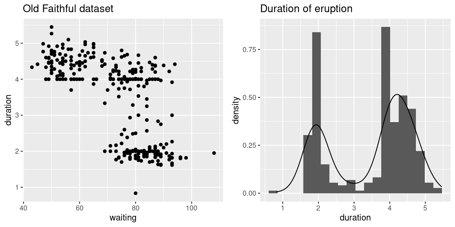
Figure 13.1: Variables in the geyser dataset.

The question of interest now is to quantify how many groups there are in the dataset and, at the same time, being able to characterize each group of duration times. A visual inspection of the right plot in Figure 13.1 suggests that there are (at least) two different groups in the data, with means roughly at about 2 and 4, and similar standard deviations between the two groups. Note that several authors have suggested a larger number of components in this dataset (Zucchini, MacDonald, and Langrock 2016), but we will only consider the analysis with two groups for simplicity.

A simple approach is to simply split the data in two groups and fit a model with two likelihoods. For example, we can assign all eruption times with a duration lower than or equal to three to group 1 and the other observations to group 2. Alternatively, the K-means algorithm can be used to obtain an initial rough classification of the data. In this particular case, both approaches will create the same initial classification of the data. Note that the response needs to be put into a 2-column matrix because two different likelihoods will be used, as described in Chapter 6.

#Index of group 1
idx1 <- geyser$duration <=3

This index will be used later to create the dataset, but it can be used now to show the number of observations assigned to each group:

table(idx1)

## idx1
## FALSE  TRUE 
##   192   107

Note how most of the observations are in the second group, as shown in Figure 13.1. The response to be used with INLA is created as follows:

# Empty response
yy <- matrix(NA, ncol = 2, nrow = nrow(geyser))

#Add data
yy[idx1, 1] <- geyser$duration[idx1]
yy[!idx1, 2] <- geyser$duration[!idx1]

Because we want each group to have a different mean, the intercept must be split in two using a similar structure to that of the observed data. In this case a 2-column matrix will be used with entries 1 and NA.

#Create two different intercepts
II <- yy
II[II > 0] <- 1

Next, the model can be fit by using values yy and I in the data (which are named duration and Intercept, respectively, in the call to inla()) and two likelihoods:

#Fit model with INLA
geyser.inla <- inla(duration ~ -1 + Intercept,
  data = list(duration = yy, Intercept = II), 
  family = c("gaussian", "gaussian"))
summary(geyser.inla)

## 
## Call:
##    c("inla(formula = duration ~ -1 + Intercept, family = 
##    c(\"gaussian\", ", " \"gaussian\"), data = list(duration = yy, 
##    Intercept = II))" ) 
## Time used:
##     Pre = 0.458, Running = 0.129, Post = 0.192, Total = 0.778 
## Fixed effects:
##             mean    sd 0.025quant 0.5quant 0.975quant  mode kld
## Intercept1 1.999 0.030      1.941    1.999      2.058 1.999   0
## Intercept2 4.275 0.027      4.222    4.275      4.328 4.275   0
## 
## Model hyperparameters:
##                                             mean    sd 0.025quant 0.5quant
## Precision for the Gaussian observations    10.71 1.458       8.08    10.64
## Precision for the Gaussian observations[2]  7.23 0.736       5.87     7.20
##                                            0.975quant  mode
## Precision for the Gaussian observations         13.79 10.51
## Precision for the Gaussian observations[2]       8.76  7.15
## 
## Expected number of effective parameters(stdev): 2.02(0.001)
## Number of equivalent replicates : 148.35 
## 
## Marginal log-Likelihood:  -140.45

The summary of the model shows that the means of the two groups have estimates 1.9994 and 4.2753, respectively. In addition, the first group has an estimated precision of 10.712, while the second has an estimated precision of 7.2257, which makes the eruptions times in the second group slightly more variable.

Although this approach leads to reasonable estimates of the eruptions times between the two groups it has two problems. The first one is that we have already used the data once to determine that there are two groups and how these two groups are defined. Secondly, this approach ignores the inherent uncertainty about from which group each observation comes. This is an important issue when classifying observations into groups and a simple cutoff point is seldom a good idea.

From a modeling point a few, what we have just done is fitting a model conditional on the auxiliary variable \(\mathbf{z}\), i.e., we have set \(\mathbf{z}\) to a given classification. Although this may be useful in practice (see Gómez-Rubio and Palmí-Perales 2019 for some examples on fitting conditional models with INLA), in a full Bayesian analysis we should also be interested in the posterior distribution of \(\mathbf{z}\).

13.3 Fitting mixture models with INLA

Mixture models are hard to fit in general (Celeux, Merrilee, and Robert 2000) and they do not fall into the class of models that INLA can fit as they cannot be expressed as a latent GMRF. However, as noted in Gómez-Rubio and HRue (2018) and Gómez-Rubio (2017) conditional on \(\mathbf{z}\) a mixture model becomes a model that can be fit with INLA.

Gómez-Rubio (2017) note that the posterior marginal of the model parameter of a mixture model can be written down as

\[ \pi(\theta_t \mid \mathbf{y}) = \sum_{z\in\mathcal{Z}} \pi(\theta_t \mid \mathbf{y},\mathbf{z}=z) \pi(\mathbf{z}= z \mid \mathbf{y}),\ t=1,\ldots, \textrm{dim}(\bm\theta) \]

Note that this requires the posterior distribution of \(\mathbf{z}\) that is usually not known. However, this can be easily estimated using INLA within MCMC, as shown in Gómez-Rubio and HRue (2018).

In this example, the Metropolis-Hastings algorithm will be used to estimate the posterior distribution of \(\mathbf{z}\). Hence, a proposal distribution is required to propose new values of \(\mathbf{z}\) and all of the assignments will be accepted or rejected as a single block (i.e., there is not individual acceptance or rejection for each \(z_i,i=1,\ldots,n\)).

The proposal distribution \(q(\mathbf{z}^{\prime} \mid \mathbf{z})\) defines the probability of a new value \(\mathbf{z}^{\prime}\) given the current value \(\mathbf{z}\). This is taken so that the probability of each individual \(z_i\) being 1 is (Marin, Mengersen, and Robert 2005)

\[ P(z_i^{\prime}=1 \mid \mathbf{z}) = \frac{w_1 f_1(y_i \mid \mu_1,\tau_1)}{w_1 f_1(y_i \mid \mu_1,\tau_1) + w_2 f_2(y_i \mid \mu_2,\tau_2)} \]

\[ P(z_i^{\prime}=2 \mid \mathbf{z}) = 1 - P(z_i^{\prime}=1 \mid \mathbf{z}) \]

Here, \(f_1(\cdot \mid \mu_1, \tau_1)\) is Normal distribution with mean \(\mu_1\) and precision \(\tau_2\), which are the ones for group 1 obtained from fitting the model conditional to \(\mathbf{z}\). \(f_2(\cdot \mid \mu_2, \tau_2)\) is defined analogously. Note that the values of the means and precisions here depend on \(\mathbf{z}\).

The example developed here is taken from Gómez-Rubio and HRue (2018) as the associated code available from https://github.com/becarioprecario/INLAMCMC_examples, which relies on function INLAMH() from package INLABMA. See Chapter 11 for details on how to fit new models with INLA by using the Metropolis-Hastings algorithm.

The different functions required to fit a mixture model using INLA within MCMC are described below. In order to have an overview of the overall picture, the different functions needed to implement this algorithm are:

get.probs(): compute the weights of the different components given an observed value of the latent variable \(\mathbf{z}\).
dq.z(): density probability function of the proposal distribution.
rq.z(): random number generator function from the proposal distribution.
fit.inla.internal(): fits the required INLA model given the value of \(\mathbf{z}\). This is used to compute the conditional marginal likelihood \(\pi(\mathbf{y} \mid \mathbf{z}\) required to compute the acceptance probability.
prior.z() computes the prior of \(\mathbf{z}\).

Also, note that the variable that stores the classification of the observations in the functions below is not simply a vector with the groups to which the observation belongs, but a more complex data structure. In particular, it is a list with the following elements:

z: Vector that indicates to which observation belongs.
m: Model fit with INLA conditional on the value of \(\mathbf{z}\). It is a list of two components: model with the INLA model fit and mlikwith the marginal likelihood of the model fit.

Note that this type of object is returned, for example, by function rq.z(). This is the data structure used to represent variable \(\mathbf{z}\) and it is passed to several functions for the computations. The reason to include the model fit is to avoid fitting it more than once in the implementation of the Metropolis-Hastings algorithm.

Before describing the required functions, the number of groups to be used is 2, which is set in variable n.grp to be used by some of the functions defined below. Also, variable grp is defined as a vector to store the initial groups to which observations belong:

# Number of groups
n.grp <- 2

# Initial classification
grp <- rep(1, length(geyser$duration))
grp[!idx1] <- 2

Function fit.inla.internal() is used to actually fit the required model given z and it is used inside rq.z() below. Note that another similar function inla.fit() is defined below for a similar purpose. The main difference between these two functions is that fit.inla.internal() is the one that calls inla() to fit the conditional model on z and that fit.inla() simply takes the fit model from the complex data structure that represents the value of z and the model fit.

#y: Vector of values with the response.
#grp: Vector of integers with the allocation variable.
fit.inla.internal <- function(y, grp) {

  #Data in two-column format
  yy <- matrix(NA, ncol = n.grp, nrow = length(y))
  for(i in 1:n.grp) {
    idx <- which(grp == i)
    yy[idx, i] <- y[idx]
  }

  #X stores the intercept in the model
  x <- yy
  x[!is.na(x)] <- 1
  
  d <- list(y = yy, x = x)

  #Model fit (conditional on z)
  m1 <- inla(y ~ -1 + x, data = d,
    family = rep("gaussian", n.grp),
    #control.fixed = list(mean = list(x1 = 2, x2 = 4.5), prec = 1)
    control.fixed = list(mean = prior.means, prec = 1)
  )

  res<- list(model = m1, mlik = m1$mlik[1, 1])
  return(res)
}

The initial data structure to represent the assignment to groups and the associated model fit (as described above) is defined next in variable grp.init. Note that given that this includes the model fit the prior means of the Gaussian prior distributions on the group means are defined through variables prior.means. Also, variable scale.sigma is set to be used in the proposal distribution.

y <- geyser$duration

prior.means <- list(x1 = 2, x2 = 4.5)
scale.sigma <- 1.25
grp.init <- list(z = grp, m = fit.inla.internal(y, grp))

Below, the functions required for the implementation of the Metropolis-Hastings algorithm are shown. Some information about their respective parameters is given as R comments.

Function get.probs() will compute the weights for each component given the current value of \(\mathbf{z}\), which is passed as a vector of integers from 1 to \(K\).

#Probabilities of belonging to each group
#z: Vector of integers with values from 1 to the number of groups
get.probs <- function(z) {
  probs <- rep(0, n.grp)
  tab <- table(z)
  probs[as.integer(names(tab))] <- tab / sum(tab)
  return(probs)
}

Next, we define function dq.z() to compute the density of a new value (z.new) of \(\mathbf{z}\) given the current one (z.old). Note that these values are a data structure as described above and not simply a vector of integers.

#Using means of conditional marginals
#FIXME: We do not consider possble label switching here
#z.old: Current value of z.
#z.new: Proposed value of z.
#log: Compute density in the log-scale.
dq.z <- function(z.old, z.new, log = TRUE) {
  m.aux <- z.old$m$model 
  means <- m.aux$summary.fixed[, "mean"]
  precs <- m.aux$summary.hyperpar[, "mean"]

  ww <- get.probs(z.old$z)

  z.probs <- sapply(1:length(y), function (X) {
    aux <- ww * dnorm(y[X], means, scale.sigma * sqrt(1 / precs))
    (aux / sum(aux))[z.new$z[X]]
  })

  if(log) {
    return(sum(log(z.probs)))
  } else {
    return(prod(z.probs))
  }
}

The function to sample random observations of \(\mathbf{z}\) using the proposal distribution given the current value of \(\mathbf{z}\), z, is rq.z(). Note that z is a complex data structure that includes the vector of indicators and the model fit, as described above.

#FIXME: We do not consider possible label switching here
#z: Current value of z.
rq.z <- function(z) {
  m.aux <- z$m$model 
  means <- m.aux$summary.fixed[, "mean"]
  precs <- m.aux$summary.hyperpar[, "mean"]

  ws <- get.probs(z$z)

  z.sim <- sapply(1:length(z$z), function (X) {
    aux <- ws * dnorm(y[X], means, scale.sigma * sqrt(1 / precs))
    sample(1:n.grp, 1, prob = aux / sum(aux))
  })

  #Fit model
  z.model <- fit.inla.internal(y, z.sim)

  #New value
  z.new <- list(z = z.sim, m = z.model)

  return(z.new)
}

The prior distribution on \(\mathbf{z}\) is simply the product of Bernoullis with probability \(0.5\) to provide a vague prior:

#z: Vector of integer values from 1 to K.
prior.z <- function(z, log = TRUE) {

  res <- log(1 / n.grp) * length(z$z)
  if(log) {
    return(res)
  }
  else {
    return(exp(res))
  }
}

Function fit.inla() is the function used by INLAMH() to fit the model given the value pf z. In this particular implementation, the actual model fitting is done inside function rq.z() using function fit.inla.internal(), so that fit.inla() simply retrieves element m from the data structure:

fit.inla <- function(y, grp) {
  return(grp$m)
}

Next, we need to call function INLAMH() to fit the model. Given that the starting point is close to the optimal partition of the data (but note that this is not usual), it is not necessary to have a large number of burn-in iterations. Furthermore, the number of iterations is kept low to 100 (after thinning one in five) because in this particular example there are only a few observations that may have a posterior probability which is not close to zero or one. In more complex examples the number of simulations is probably required to be higher.

#Run simulations
library("INLABMA")
inlamh.res <- INLAMH(geiser$duration, fit.inla, grp.init, rq.z, dq.z, 
  prior.z, n.sim = 100, n.burnin = 20, n.thin = 5, verbose = TRUE)

Once the model has been fit, it will return a list with the fitted models and the values of \(\mathbf{z}\) (that includes many auxiliary variables that are not actually needed). The sampled values of \(\mathbf{z}\) are obtained as

zz <- do.call(rbind, lapply(inlamh.res$b.sim, function(X){X$z}))

From this sample from the posterior distribution \(\pi(\mathbf{z} \mid \mathbf{y})\) we can compute the posterior probabilities of belonging to each group:

zz.probs <- apply(zz, 2, get.probs)

Note that probabilities for most observations are 0 and 1, i.e., classification is quite clear, and only a few observations will show some uncertainty in the classification. Figure 13.2 shows the observed values against the posterior probabilities of belonging to the group of eruptions with the lower durations (i.e., \(z_i=1\)).

The conditional marginal likelihoods of all the models associated with the sampled values of \(\mathbf{z}\) can also be obtained to gain some insight on the simulation process:

mliks <- do.call(rbind, lapply(inlamh.res$model.sim, function(X){X$mlik}))

These are also shown in Figure 13.2 (right plot) and they show how the sampling algorithm produces an increase of the conditional marginal likelihoods as compared to the initial model fit above in Section 13.2 (which had a marginal likelihood of -140.16). This also means that the short burn-in period is enough.

Furthermore, the chain shows that only a few classifications are explored. This behavior can be easily changed by increasing the number of iterations for thinning or choosing a different proposal distribution, for example, one that takes higher values of the standard deviations (e.g., twice their values). However, in this particular case most of the observations have high posterior probabilities of belonging to one of the two groups, which means that they are always classified in the same group. Hence, the posterior probabilities are accumulated in a few classifications where only the observations with a duration time of about 3 minutes are classified in either of the two groups.

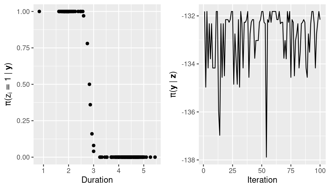
Posterior probabilities of the observed data (left) and conditional marginal likelihood (right) of the model fit to the duration of geyser eruptions (in minutes).

Figure 13.2: Posterior probabilities of the observed data (left) and conditional marginal likelihood (right) of the model fit to the duration of geyser eruptions (in minutes).

13.4 Model selection for mixture models

Determining the number of components in a model is often difficult and a number of proposals have been made so far. Here we will simply approach the estimation of the marginal likelihood of the mixture model with a known number of groups by noting that it can be computed as (Gómez-Rubio 2017):

\[ \pi(\mathbf{y}) = \sum_{z\in\mathcal{Z}} \pi(\mathbf{y} \mid \mathbf{z}=z) \pi(\mathbf{z} = z) \]

Note that \(\pi(\mathbf{y} \mid \mathbf{z}=z)\) can be approximated with accuracy by the marginal likelihood returned by fitting a model with INLA given \(\mathbf{z}\). Furthermore, \(\pi(\mathbf{z})\) is the prior distribution which is always known.

Alternatively, the marginal likelihood of a mixture model can be computed by noting that (Chib 1995):

\[ \pi(\mathbf{y}) = \frac{\pi(\mathbf{y} \mid \mathbf{z} = z^*)\pi(\mathbf{z} = z^*)}{\pi(\mathbf{z} = z^*) \mid \mathbf{y})},\ z^*\in\mathcal{Z} \]

Note that in order to make the previous computation stable the posterior probability of \(z^*\) must be bounded away from zero. A good choice would be the posterior mode of \(\mathbf{z}\).

For example, we can take the value of \(\mathbf{z}\) with the highest marginal likelihood (note that all values of z have the same value of the prior), which is the one obtained at iteration 60:

z.idx <- 60

Then, the estimate of the conditional marginal likelihood \(\pi(\mathbf{y} \mid \mathbf{z} = z^*)\) provided by INLA is

#Marginal likelihood (log-scale)
mliks[z.idx]

## [1] -131.8

Next, the prior at the \(z^*\), \(\pi(\mathbf{z} = z^*)\), is computed as

#Prior (log-scale)
prior.z(inlamh.res$b.sim[[z.idx]])

## [1] -207.3

Finally, the posterior probability of \(z^*\) is obtained from the sample from the posterior distribution of \(\mathbf{z}\) obtained from the MCMC algorithm. This is done by simply checking the proportion of times \(z^*\) appears in the sample from the posterior distribution of \(\mathbf{z}\):

#Posterior probabilities
z.post <- table(apply(zz, 1, function(x) {paste(x, collapse = "")})) / 100

# Get post. prob. of z^* in the log-scale
log.pprob <- unname( 
  log(z.post[names(z.post) ==
    paste(inlamh.res$b.sim[[z.idx]]$z, collapse = "")])
)
log.pprob

## [1] -1.561

Note that the paste() function has been used above in order to create an unique label for each value of \(\mathbf{z}\) by appending all its values together. The resulting label has the same length of the number of observations and it can be very long. In any case, this is a simple way to identify each value of the latent variable with a label, although shorter options should be preferred in practice (such as hash tables). Having an unique label for each value of \(\mathbf{z}\) allows us to use the table() function on the sample values directly to compute the number of times each value of the latent variable appears in the MCMC sample.

Hence, the estimate of the marginal likelihood (in the log-scale) is

mlik.mix <- mliks[z.idx] + prior.z(inlamh.res$b.sim[[z.idx]]) - log.pprob
mlik.mix

## [1] -337.5

Note that this estimate of the marginal likelihood relies on the approximations to \(\pi(\mathbf{y} \mid \mathbf{z} = z^*)\) (which is provided by INLA) and \(\pi(\mathbf{z} = z^* \mid \mathbf{y})\) (which is obtained from the MCMC samples). Hence, in order to obtain reliable estimates it may be required to run the MCMC algorithm for a longer number of iterations.

This value of the marginal likelihood obtained can be compared to the one reported by INLA when a Gaussian model with a single likelihood is fit to the whole dataset:

inla(duration ~ 1, data = geyser)$mlik[1,1]

## log marginal-likelihood (integration) 
##                                -478.6

Finally, the same approach can be used to fit a model with three components to the data. This will require setting the number of groups to three and generating a suitable starting point (which in this case is splitting the data into three groups of equal size):

#Number of groups 
n.grp <- 3

#Initial classification
grp3 <- as.numeric(cut(geyser$duration, 3))
grp.init3 <- list(z = grp3, m = fit.inla.internal(y, grp3))

Next, the prior means and scale of the standard deviation of the proposal distribution are set:

#Priors for  the means
prior.means <- list(x1 = 2, x2 = 3.5, x3 = 5)
#Scale st. dev. of proposal distribution
scale.sigma <- 1

Once all parameters have been defined to fit a mixture model with three components, model fitting is carried out with the INLAMH() function:

inlamh.res3 <- INLAMH(geiser$duration, fit.inla, grp.init3, rq.z, dq.z, 
  prior.z, n.sim = 100, n.burnin = 20, n.thin = 5, verbose = TRUE)

Then, the marginal likelihood of this mixture model with three components can be computed similarly as before. First, the value of \(\mathbf{z}\) with the largest conditional marginal likelihood (\(z^*\)) is obtained:

##Conditional (on z) marg. lik.
mliks3 <- do.call(rbind, lapply(inlamh.res3$model.sim, function(X){X$mlik}))
#z^* with maximum cond. marg. lik.
z.idx3 <- which.max(mliks3)

Next, the log-posterior probability of \(z^*\) is estimated from the MCMC sample:

#Get all values of z in the sample
zz3 <- do.call(rbind, lapply(inlamh.res3$b.sim, function(X){X$z}))
#Table of posterior probabilities
z.post3 <- table(apply(zz3, 1, function(x) {paste(x, collapse = "")})) / 100

#Log-posterior probability of z^*
log.pprob3 <- unname(
  log(z.post3[names(z.post3) == paste(inlamh.res3$b.sim[[z.idx3]]$z,
     collapse = "")])
)

Finally, the marginal likelihood is estimated by combining these two values with the prior probability of \(z^*\):

#Marginal likelihood 
mlik.mix3 <- mliks3[z.idx3] + prior.z(inlamh.res3$b.sim[[z.idx3]]) -
  log.pprob3
mlik.mix3

## [1] -291.4

Note how the estimate of the marginal likelihood obtained now is larger than for the models with 1 and 2 components. This means that there are probably (at least) three groups in the data and not two, as discussed in Zucchini, MacDonald, and Langrock (2016).

In order to summarize the fit model using the model with 2 and 3 components, Figure 13.3 shows the mixture using the posterior means of the model parameter. Function inla.merge() will be used to merge all the models obtained in the Metropolis-Hastings algorithms. This will provide the posterior means of the means and precisions in the model. The posterior means of weights \(\mathbf{w}\) will be obtained from the posterior mean of the proportions of observations in each group (which assumes a very vague flat prior).

#Merge models
models <- lapply(inlamh.res$model.sim, function(X) {X$model})
mix.model <- inla.merge(models)

#Post. means
mix.means <- mix.model$summary.fixed[, "mean"]
mix.precs <- mix.model$summary.hyperpar[, "mean"]

#Post. means of weights
n.grp <- 2
mix.w <- apply(apply(zz, 1, get.probs), 1, mean)

Similarly, for the model with 3 components:

#Merge models
models3 <- lapply(inlamh.res3$model.sim, function(X) {X$model})
mix.model3 <- inla.merge(models3)

#Post. means
mix.means3 <- mix.model3$summary.fixed[, "mean"]
mix.precs3 <- mix.model3$summary.hyperpar[, "mean"]

#Post. means of weights
n.grp <- 3
mix.w3 <- apply(apply(zz3, 1, get.probs), 1, mean)

Figure 13.3: Mixtures estimated at the posterior mode of z using the posterior means of the parameters for the models with 2 and 3 groups.

13.5 Cure rate models

Survival models described in Chapter 10 assume that all subjects will eventually experience the event of interest. However, in some situations subjects may get cured and, hence, will not be susceptible to experience this event. A typical situation is a patient who is cured from a disease after receiving proper treatment.

This situation can be conveniently represented by a mixture model with two groups: a group of cured subjects and a group of non-cured that have experienced the event or that will eventually. This is a particular type of mixture model with only two classes. Furthermore, some of the subjects will automatically be assigned to the second group as they have already experienced the event. This makes cure rate models easier to identify as these subjects will help to identify the second group, which in turn will help to identify the first group.

In INLA, cure rate models are represented by a constant density (equal to 1) for the first group and a Weibull density for the second group. See inla.doc("weibullcure") for details.

This model can be described as follows:

\[ y_i \mid w,\bm\theta \sim w \cdot 1 + (1 - w) f(y_i \mid \bm\theta),\ i = 1,\ldots, n \]

Here, \(f(\cdot \mid \theta)\) represents a Weibull distribution and its parameterization in INLA is:

\[ f(y_i \mid \alpha) = \alpha y_i^{\alpha - 1} \lambda \exp\{-\lambda y_i^{\alpha}\}. \]

Note that this parameterization of the Weibull distribution is similar to the variant=0 of the Weibull family available in likelihood weibull. See inla.doc("weibullcure") for details.

In the equation above, \(y_i\) represent survival times and it is a non-negative variable, \(\alpha\) is a positive shape parameter and \(\lambda\) is a parameter that is linked to the linear predictor. This link is as follows:

\[ \lambda = \exp(\eta) \] where \(\eta\) is the linear predictor.

Priors for this model are defined on the internal representation of parameters \(\alpha\) and \(w\). In particular, the internal parameterization is

\[ \theta_1 = \log(\alpha) \]

\[ \theta_2 = \log(\frac{w}{1 - w}) \]

This parameterization makes sure that \(\theta_1\) and \(\theta_2\) are not in a bounded interval, which simplifies optimization and model fitting. The default prior on \(\theta_1\) is a log-gamma with parameters 25 and 25, while the prior on \(\theta_2\) is Gaussian with mean -1 and precision 0.2. These priors can be changed as described in Chapter 5.

Package smcure (Cai et al. 2012 a, 2012 b) provides dataset e1684 from the Eastern Cooperative Oncology Group (ECOG) phase III clinical trial e1684 (see, Kirkwood et al. 1996, for details). The clinical trial was conducted to test whether Interferon alpha-2b (IFN alpha-2b) exhibits antitumor activity in metastatic melanoma. Table 13.2 describes the variables in the dataset.

Table 13.2: Variables in the `e1684` dataset.
Variable	Description
`TRT`	Treatment (0=control, 1=IFN treatment)
`FAILTIME`	Observed relapse-free time.
`FAILCENS`	Censoring indicator (1=event happens, 0=event not observed)
`AGE`	Age of patient (centered to the mean).
`SEX`	Sex (1 for female and 0 for male).

The original dataset can be loaded as follows:

library("smcure")
data(e1684)
summary(e1684)

##       TRT           FAILTIME        FAILCENS          AGE        
##  Min.   :0.000   Min.   :0.033   Min.   :0.000   Min.   :-29.99  
##  1st Qu.:0.000   1st Qu.:0.356   1st Qu.:0.000   1st Qu.:-11.32  
##  Median :1.000   Median :1.238   Median :1.000   Median :  0.58  
##  Mean   :0.509   Mean   :2.763   Mean   :0.691   Mean   :  0.00  
##  3rd Qu.:1.000   3rd Qu.:4.956   3rd Qu.:1.000   3rd Qu.: 11.03  
##  Max.   :1.000   Max.   :9.644   Max.   :1.000   Max.   : 31.70  
##                                                  NA's   :1       
##       SEX       
##  Min.   :0.000  
##  1st Qu.:0.000  
##  Median :0.000  
##  Mean   :0.398  
##  3rd Qu.:1.000  
##  Max.   :1.000  
##  NA's   :1

In order to make summary results more informative, factors in the dataset will be assigned these labels:

#Assign labels to factors
e1684$TRT <- as.factor(e1684$TRT)
levels(e1684$TRT) <- c("Control", "IFN")

e1684$SEX <- as.factor(e1684$SEX)
levels(e1684$SEX) <- c("Female", "Male")

Finally, observation number 37 will be removed because of missing observations:

# Remove observation 37 because it has missing values
d <- na.omit(e1684)

Now, the data can be summarized as follows:

summary(d)

##       TRT         FAILTIME        FAILCENS         AGE        
##  Control:140   Min.   :0.033   Min.   :0.00   Min.   :-29.99  
##  IFN    :144   1st Qu.:0.354   1st Qu.:0.00   1st Qu.:-11.32  
##                Median :1.215   Median :1.00   Median :  0.58  
##                Mean   :2.754   Mean   :0.69   Mean   :  0.00  
##                3rd Qu.:4.950   3rd Qu.:1.00   3rd Qu.: 11.03  
##                Max.   :9.644   Max.   :1.00   Max.   : 31.70  
##      SEX     
##  Female:171  
##  Male  :113  
##              
##              
##              
##

Next, a Kaplan-Meier estimate of the survival times is obtained using function survfit() from package survival (see Chapter 10 for details):

library("survival")

km <- survfit(Surv(d$FAILTIME, d$FAILCENS) ~ 1)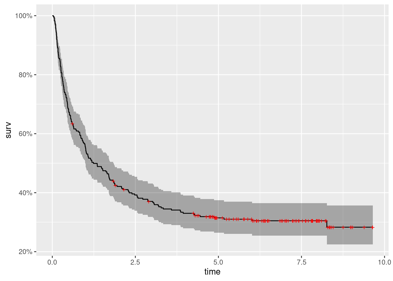

Figure 13.4: Kaplan-Meier estimate of the survival times in the e1684 dataset.

This has been plotted in Figure 13.4. Next, the model is fit. Note that first the response variable needs to be created by using function inla.surv(). See Chapter 10 for details.

d.inla <- list(y = inla.surv(d$FAILTIME, d$FAILCENS),
  Treatment = d$TRT, Age = d$AGE, Female = d$SEX)

cure.inla <- inla(y ~ Treatment + Age + Female, family = "weibullcure",
  data = d.inla)
summary(cure.inla)

## 
## Call:
##    c("inla(formula = y ~ Treatment + Age + Female, family = 
##    \"weibullcure\", ", " data = d.inla)") 
## Time used:
##     Pre = 0.214, Running = 0.252, Post = 0.0206, Total = 0.486 
## Fixed effects:
##                mean    sd 0.025quant 0.5quant 0.975quant   mode kld
## (Intercept)  -0.071 0.120     -0.314   -0.068      0.158 -0.063   0
## TreatmentIFN -0.134 0.160     -0.454   -0.132      0.176 -0.128   0
## Age          -0.007 0.006     -0.017   -0.007      0.004 -0.006   0
## FemaleMale    0.142 0.161     -0.178    0.143      0.454  0.146   0
## 
## Model hyperparameters:
##                         mean    sd 0.025quant 0.5quant 0.975quant  mode
## alpha parameter for ps 0.927 0.050      0.830    0.926      1.027 0.926
## p parameter for ps     0.297 0.028      0.244    0.296      0.353 0.295
## 
## Expected number of effective parameters(stdev): 4.00(0.00)
## Number of equivalent replicates : 70.98 
## 
## Marginal log-Likelihood:  -401.64

The estimates are similar to those reported in Lázaro, Armero, and Gómez-Rubio (2020), which compare MCMC and a different model fitting approach similar to Gibbs sampling with INLA.

Note that the cure rate model estimates that the posterior mean of the proportion of cured patients is 0.2968. A typical analysis using a Weibull survival model (i.e., ignoring the possibility of being cured) will yield the following results:

weibull.inla <- inla(y ~ Treatment + Age + Female, family = "weibullsurv",
  data = d.inla, control.family = list(list(variant = 0)))
summary(weibull.inla)

## 
## Call:
##    c("inla(formula = y ~ Treatment + Age + Female, family = 
##    \"weibullsurv\", ", " data = d.inla, control.family = 
##    list(list(variant = 0)))" ) 
## Time used:
##     Pre = 0.198, Running = 0.131, Post = 0.0201, Total = 0.349 
## Fixed effects:
##                mean    sd 0.025quant 0.5quant 0.975quant   mode kld
## (Intercept)  -0.641 0.122     -0.885   -0.639     -0.407 -0.635   0
## TreatmentIFN -0.379 0.144     -0.662   -0.379     -0.098 -0.379   0
## Age           0.007 0.005     -0.004    0.007      0.017  0.007   0
## FemaleMale    0.001 0.147     -0.290    0.002      0.286  0.003   0
## 
## Model hyperparameters:
##                                  mean    sd 0.025quant 0.5quant 0.975quant
## alpha parameter for weibullsurv 0.606 0.035       0.54    0.606      0.677
##                                  mode
## alpha parameter for weibullsurv 0.605
## 
## Expected number of effective parameters(stdev): 4.00(0.00)
## Number of equivalent replicates : 70.98 
## 
## Marginal log-Likelihood:  -433.14

Notice how the effect of the treatment is significant now. Hence, making the assumption that patients can be cured can have an important effect on the estimation of the main effects in the model. Furthermore, the marginal likelihood of the cure rate model is larger than the one of the Weibull model, which suggests a better fit of the cure rate model. However, bear in mind that the marginal likelihood does not penalize for the complexity of the model. Overfit models tend to have higher values of the marginal likelihood.

13.5.1 Joint cure rate models

When studying cure rate models also of interest is the probability of being cured for each patient. Note that a survival model will look at survival times (that may be affected by receiving a treatment) and that a cure rate model will look at the proportions of cured subjects. This probability can also be modeled on the covariates. However, the weibullcure latent effect does not allow for the inclusion of the covariates to model cure rate proportion \(w\).

Lázaro, Armero, and Gómez-Rubio (2020) propose a joint model that includes a cure rate model and a logistic regression to model \(w\). Modeling relies on introducing a latent variable \(\mathbf{z}\) to assign each subject to the cured or uncured groups. The model is fit using an algorithm similar to Gibbs sampling and at each step the survival model is fit on the uncured population and a logistic regression using the complete dataset to model \(\mathbf{z}\) on the explanatory covariates. Hence, this joint model can estimate survival times as well as the probability of being cured.

13.6 Final remarks

Here we have provided an introduction on how to use INLA to fit mixture models. This approach is based on fitting conditional models on \(\mathbf{z}\) and seems to provide good results for the examples presented herein. However, fitting mixture models is difficult in general. Furthermore, this approach relies on having good approximations to the marginal likelihoods of the conditional models, which may not always be the case (see Gómez-Rubio and HRue 2018 for a discussion on this).

On the other hand, the computational approach described here to fit mixture models with INLA has the advantage of providing a toolbox for building different types of mixture models, with different types of likelihoods and priors on the hyperparameters not restricted to conjugate priors. These are probably the two major advantages of this approach.

References

Azzalini, A., and A. W. Bowman. 1990. “A Look at Some Data on the Old Faithful Geyser.” Applied Statistics 39: 357–65.

Cai, Chao, Yubo Zou, Yingwei Peng, and Jiajia Zhang. 2012a. “Smcure: An R-Package for Estimating Semiparametric Mixture Cure Models.” Computer Methods and Programs in Biomedicine 108 (3): 1255–60.

Cai, Chao, Yubo Zou, Yingwei Peng, and Jiajia Zhang. 2012b. Smcure: Fit Semiparametric Mixture Cure Models. https://CRAN.R-project.org/package=smcure.

Carlin, Bradley P., and Siddhartha Chib. 1995. “Bayesian Model Choice via Markov Chain Monte Carlo Methods.” Journal of the Royal Statistical Society, Series B 57 (3): 473–84.

Celeux, Gilles, Merrilee, and Christian P. Robert. 2000. “Computational and Inferential Difficulties with Mixture Posterior Distributions.” Journal of the American Statistical Association 95 (451): 957–70.

Chib, S. 1995. “Marginal Likelihood from the Gibbs Output.” Journal of the American Statistical Association 90 (432): 1313–21.

Dempster, A. P., N. M. Laird, and D. B. Rubin. 1977. “Maximum Likelihood from Incomplete Data via the EM Algorithm (with Discussion).” Journal of the Royal Statistical Society: Series B 39: 1–38.

Diebolt, Jean, and Christian P. Robert. 1994. “Estimation of Finite Mixture Distributions Through Bayesian Sampling.” Journal of the Royal Statistical Society, Series B 56 (2): 363–75.

Frühwirth-Schnatter, Sylvia, Gilles Celeux, and Christian P. Robert, eds. 2018. Handbook of Mixture Analysis. Boca Raton, FL: Chapman & Hall/CRC Press.

Gómez-Rubio, Virgilio. 2017. “Mixture model fitting using conditional models and modal Gibbs sampling.” arXiv E-Prints, December, arXiv:1712.09566. http://arxiv.org/abs/1712.09566.

Gómez-Rubio, Virgilio, and HRue. 2018. “Markov Chain Monte Carlo with the Integrated Nested Laplace Approximation.” Statistics and Computing 28 (5): 1033–51.

Gómez-Rubio, Virgilio, and Francisco Palmí-Perales. 2019. “Multivariate Posterior Inference for Spatial Models with the Integrated Nested Laplace Approximation.” Journal of the Royal Statistical Society: Series C (Applied Statistics) 68 (1): 199–215. https://doi.org/10.1111/rssc.12292.

Kirkwood, J M, M H Strawderman, M S Ernstoff, T J Smith, E C Borden, and R H Blum. 1996. “Interferon Alfa-2b Adjuvant Therapy of High-Risk Resected Cutaneous Melanoma: The Eastern Cooperative Oncology Group Trial Est 1684.” Journal of Clinical Oncology 14 (1): 7–17. https://doi.org/10.1200/JCO.1996.14.1.7.

Lázaro, Elena, Carmen Armero, and Virgilio Gómez-Rubio. 2020. “Approximate Bayesian inference for mixture cure models.” TEST, to appear.

Marin, Jean-Michel, Kerrie Mengersen, and Christian P. Robert. 2005. “Bayesian Modelling and Inference on Mixtures of Distributions.” In Handbook of Statistics, edited by D K. Dey and C. R. Rao. Vol. 25. Elsevier.

Richardson, Sylvia., and Peter J. Green. 1997. “On Bayesian Analysis of Mixtures with an Unknown Number of Components (with Discussion).” Journal of the Royal Statistical Society: Series B (Statistical Methodology) 59 (4): 731–92. https://doi.org/10.1111/1467-9868.00095.

Stephens, Matthew. 2000. “Dealing with Label Switching in Mixture Models.” Journal of the Royal Statistical Society: Series B (Statistical Methodology) 62 (4): 795–809. https://doi.org/10.1111/1467-9868.00265.

Zucchini, W., I. L. MacDonald, and R. Langrock. 2016. Hidden Markov Models for Time Series: An Introduction Using R. 2nd ed. CRC Press.