Chapter 3 Mixed-effects Models

3.1 Introduction

In Chapter 2 we have already introduced how to fit models with fixed and random effects. In this chapter a more detailed description of the different types of fixed and random effects available in INLA will be provided.

First of all, let’s recall that a covariate should enter the model as a linear fixed effect when it is thought that it affects all observations in the same way (in a linear way, in fact) and that this effect is of primary interest in the study.

Random effects, on the other hand, are often adopted to take into account variation produced by variables in the model that are not our primary object of study. For example, in a study to investigate the effect of different irrigation systems on plant growth, measurement may include the type of irrigation, type of soil and variables associated with the trees, such as a numerical identifier of the tree, age, etc. Trees themselves in the study are not the primary object of study as they are a (random) sample of the population of trees. However, depending on the actual tree being measured, growth may be faster or slower and it will affect the growth measurement. In this case, because the trees in the study are taken as a random sample from the total population of trees, their effect is included as a random effect.

In a Bayesian context, a fixed effect will have an associated coefficient which is often assigned a vague prior, such as a Gaussian with zero mean and large variance. On the other hand, random effects will have a common Gaussian prior with a zero mean and a precision, to which a prior will be assigned.

3.2 Fixed-effects models

As explained in Section 2.3, fixed effects can be easily included in the model formula. The default prior assigned to the associated coefficients (and the intercept) is a Gaussian distribution, and its parameters can be set through option control.fixed in the call to inla().

Fixed effects can also be included in the model by including one or more terms in the model formula using the the f() function. Table 3.1 summarizes the two types of fixed effects implemented in INLA, which will be described in more detail below.

Table 3.1: Summary of types of fixed effects implemented in INLA.

Name	Description
linear	Linear fixed effect.
clinear	Linear fixed effect with constrained coefficient.

3.2.1 linear fixed effect

The linear effect is similar to including a covariate in the formula in the usual way and it implements the effect \(\beta x_i\), where \(x_i\) is the value of the covariate for observation \(i\) and \(\beta\) the associated coefficient. The prior on \(\beta\) is a Gaussian distribution with mean and precision that can be specified in the call to the f() function when the model is defined in the formula. Table 3.2 summarizes the specific options available for this effect. Alternatively, parameter control.fixed can be used to set the prior on the coefficient.

Table 3.2: Summary of options of the linear effect.

Argument	Default	Description
mean.linear	\(0\)	Mean of Gaussian prior on a coefficient.
prec.linear	\(0.001\)	Precision of Gaussian prior on a coefficient.

3.2.2 clinear fixed effect

Sometimes it is necessary to fit a model in which the covariate coefficients are constrained in some way, e.g., we want to force the coefficient to be non-negative. This can be achieved by means of the clinear effect. Table 3.3 shows the different options available to specify this effect. Note that precision is the precision of a (tiny) error that is added to the actual value of \(\beta x_i\) required by how this latent effect is implemented.

Table 3.3: Summary of options of the clinear effect.

Argument	Default	Description
range	c(-Inf, Inf)	Vector of length two with the range of the linear coefficient.
precision	exp(14)	Tiny precision to implement this latent effect.

The implementation of this effect distinguishes three different possibilities depending on how range is defined:

• range = c(-Inf, Inf)

  In this case there are not constraints and the model is equivalent to the linear effect. The parameterization is \(\beta = \theta\), where \(\theta\) is the parameter in the internal scale used by INLA to estimate the model.

• range = c(a, Inf)

  In this case a is the lower bound of the parameter and there is no upper limit, so the internal parameterization is

  \[ \beta = a + \exp(\theta) \]

• range = c(a, b)

  This is the model general case in which both limits, lower bound a and upper bound b, are real numbers. The internal parameterization is now:

  \[ \beta = a + (b - a) \frac{\exp(\theta)}{1 + \exp(\theta)} \]

In all cases the prior of this model is set on the internal parameter \(\theta\) and it is a Gaussian distribution with default mean equal to 1 and precision equal to 10.

In order to illustrate the use of the two models for fixed effects we will revisit the example on the SIDS dataset. A model will be fitted to constrain to a positive coefficient on the covariate that represents the proportion of non-white births in a county.

First of all, the dataset will be loaded and the required variables computed (see Chapter 2 for details):

library("spdep")
data(nc.sids)

# Overall rate
r <- sum(nc.sids$SID74) / sum(nc.sids$BIR74)
nc.sids$EXP74 <- r * nc.sids$BIR74

# Proportion of non-white births
nc.sids$NWPROP74 <- nc.sids$NWBIR74 / nc.sids$BIR74

Next, the two models will be fitted. First of all, the model using the linear effect:

m.pois.lin1 <- inla(SID74 ~ f(NWPROP74, model = "linear"),
  data = nc.sids, family = "poisson", E = EXP74)

summary(m.pois.lin1)

## 
## Call:
##    c("inla(formula = SID74 ~ f(NWPROP74, model = \"linear\"), family 
##    = \"poisson\", ", " data = nc.sids, E = EXP74)") 
## Time used:
##     Pre = 0.352, Running = 0.0592, Post = 0.0201, Total = 0.432 
## Fixed effects:
##               mean    sd 0.025quant 0.5quant 0.975quant   mode kld
## (Intercept) -0.646 0.090     -0.824   -0.645     -0.470 -0.644   0
## NWPROP74     1.869 0.217      1.440    1.869      2.293  1.870   0
## 
## Expected number of effective parameters(stdev): 2.00(0.00)
## Number of equivalent replicates : 49.90 
## 
## Marginal log-Likelihood:  -226.12

Note how the posterior marginal of the coefficient of covariate NWPROP74 has a 95% credible interval which is above zero. In case we wanted this coefficient to be positive, this is how the model with a constraint on the coefficient using the clinear effect is fitted:

library("INLA")
m.pois.clin1 <- inla(SID74 ~ f(NWPROP74, model = "clinear",
  range = c(0, Inf)), data = nc.sids, family = "poisson",
  E = EXP74)

summary(m.pois.clin1)

## 
## Call:
##    c("inla(formula = SID74 ~ f(NWPROP74, model = \"clinear\", range = 
##    c(0, ", " Inf)), family = \"poisson\", data = nc.sids, E = EXP74)" 
##    ) 
## Time used:
##     Pre = 0.211, Running = 0.0923, Post = 0.0211, Total = 0.324 
## Fixed effects:
##               mean    sd 0.025quant 0.5quant 0.975quant   mode   kld
## (Intercept) -0.672 0.084     -0.843    -0.67     -0.514 -0.666 0.002
## 
## Random effects:
##   Name     Model
##     NWPROP74 Constrained linear
## 
## Model hyperparameters:
##                   mean   sd 0.025quant 0.5quant 0.975quant mode
## Beta for NWPROP74 1.93 0.20       1.54     1.93       2.33 1.93
## 
## Expected number of effective parameters(stdev): 1.00(0.00)
## Number of equivalent replicates : 99.55 
## 
## Marginal log-Likelihood:  -222.89

It can be seen how the estimates of the intercept and the coefficient of the proportion of non-white births are very similar between the unconstrained and the constrained model.

3.3 Types of mixed-effects models

The list of random effects implemented in INLA is quite rich. Random effects in INLA are defined using a multivariate Gaussian distribution with zero mean and precision matrix \(\tau \Sigma\), where \(\tau\) is a generic precision parameter and \(\Sigma\) is a matrix that defines the dependence structure of the random effects and that may depend on further parameters. When the random effects are a latent Gaussian Markov random field the structure of \(\Sigma\) is quite sparse and this can be exploited for computational purposes (Rue and Held 2005). Given a vector \(\mathbf{u}\) of random effects, this will be represented as:

\[ \mathbf{u} \sim N(0, \tau \Sigma) . \]

Table 3.4 summarizes the ones described in this chapter, but other types of random effects are discussed in different chapters.

Table 3.4: Summary of some of the random effects implemented in INLA.

Name	Description
iid	Independent and identically distributed Gaussian random effect.
z	“Classical” specification of random effects.
generic0	Generic specification (type 0).
generic1	Generic specification (type 1).
generic2	Generic specification (type 2).
generic3	Generic specification (type 3).
rw1	Random walk of order 1.
rw2	Random walk of order 2.
crw2	Continuous random walk of order 2.
seasonal	Seasonal variation with a given periodicity.
ar1	Autoregressive model of order 1.
ar	Autoregressive model of arbitrary order.
iid1d	Correlated random effects of dimension 1.
iid2d	Correlated random effects of dimension 2.
iid3d	Correlated random effects of dimension 3.
iid4d	Correlated random effects of dimension 4.
iid5d	Correlated random effects of dimension 5.

3.3.1 Independent random effects (iid model)

Independent and identically distributed random effects have already been introduced in Chapter 2 and they are probably the simplest way to account for unstructured variability in the data.

The precision matrix of iid random effects is \(\tau \Sigma\) with \(\Sigma\) a diagonal matrix of scaling factors \(\{s_1, \ldots,s_n\}\) (which are all equal to 1 by default). Scaling factors are defined by means of parameter scale within the f() function used to define the latent effect in the formula.

The internal parameterization of the hyperparameter of this model is \(\theta = \log (\tau)\), which by default is assigned a log-Gamma distribution with parameters \(1\) and \(0.00005\). In other words, the prior of \(\tau\) is a Gamma distribution.

The first argument passed to the f() function should be an index of values that define the grouping of the observations in order to define the number of random effects. The length of parameter scale, if used, must be equal to the number of groups defined. Scaling may be used, for example, to account for different sample sizes in the groups defined by the data (see Section 5.6).

This type of random effects is often used to account for overdispersion in Poisson models. For this reason, the example will be again based on the SIDS dataset. The first step is to create an index for the random effects:

nc.sids$ID <- 1:100

Here, the index goes from 1 to 100 because we want a different value of the random effect for each county. If different counties must share the same random effect then the index variable should assign the same value to these counties.

The iid is then added to the model formula, using the f() function:

m.pois.iid <- inla(SID74 ~ f(ID, model = "iid"),
  data = nc.sids, family = "poisson",
  E = EXP74)

summary(m.pois.iid)

## 
## Call:
##    c("inla(formula = SID74 ~ f(ID, model = \"iid\"), family = 
##    \"poisson\", ", " data = nc.sids, E = EXP74)") 
## Time used:
##     Pre = 0.211, Running = 0.143, Post = 0.0191, Total = 0.374 
## Fixed effects:
##               mean    sd 0.025quant 0.5quant 0.975quant   mode kld
## (Intercept) -0.028 0.063     -0.155   -0.026      0.092 -0.024   0
## 
## Random effects:
##   Name     Model
##     ID IID model
## 
## Model hyperparameters:
##                  mean   sd 0.025quant 0.5quant 0.975quant mode
## Precision for ID 7.26 2.57       3.79     6.77      13.61 6.02
## 
## Expected number of effective parameters(stdev): 40.44(6.52)
## Number of equivalent replicates : 2.47 
## 
## Marginal log-Likelihood:  -245.54

The posterior mean of the precision of the random effects is 7.2609, which is a clear sign of overdispersion.

The same model can now include the covariate on the proportion of non-white births:

m.pois.iid2 <- inla(SID74 ~ NWPROP74 + f(ID, model = "iid"),
  data = nc.sids, family = "poisson",
  E = EXP74)

summary(m.pois.iid2)

## 
## Call:
##    c("inla(formula = SID74 ~ NWPROP74 + f(ID, model = \"iid\"), 
##    family = \"poisson\", ", " data = nc.sids, E = EXP74)") 
## Time used:
##     Pre = 0.212, Running = 0.117, Post = 0.0193, Total = 0.348 
## Fixed effects:
##               mean    sd 0.025quant 0.5quant 0.975quant   mode kld
## (Intercept) -0.646 0.093     -0.829   -0.645     -0.466 -0.644   0
## NWPROP74     1.871 0.224      1.431    1.871      2.310  1.872   0
## 
## Random effects:
##   Name     Model
##     ID IID model
## 
## Model hyperparameters:
##                      mean       sd 0.025quant 0.5quant 0.975quant  mode
## Precision for ID 15986.25 19485.14      14.00  9361.65   69186.70 15.69
## 
## Expected number of effective parameters(stdev): 5.04(7.11)
## Number of equivalent replicates : 19.83 
## 
## Marginal log-Likelihood:  -227.85

Now, the posterior mean of the precision of the random effects is \(1.5986\times 10^{4}\). This means that the covariate explains most of the overdispersion in the data.

3.3.2 Generic specification

In general, iid random effects are not suitable to model complex covariate structures that often appear in experimental design. For this reason, INLA provides a number of generic specifications for random effects, in addition to some specific ones (that are described later in this chapter).

3.3.3 Mixed-effects design matrix (z model)

The z latent model can be used to define a term \(Z \mathbf{u}\) in the linear predictor where \(Z\) is a defined matrix and \(\mathbf{u}\) is a vector of iid random effects with zero mean and precision \(\tau C\). \(C\) is a known matrix, and it is taken to be a diagonal matrix of the appropriate dimension if it is not specified.

This random effect allows for the following representation of the linear predictor:

\[ \eta = X \beta + Z \mathbf{u} \] which is a standard and generic representation of mixed-effects models (Pinheiro and Bates 2000). Hence, \(Z\) can be regarded as a “design matrix” for the random effects and it will allow one observation to depend on more than one random effect. Note that \(Z\) will have as many rows as observations and as many columns as elements in the vector of random effects \(\mathbf{u}\).

Because of the way this latent effect is implemented in INLA, the actual model is:

\[ \eta = Z\mathbf{u} + \varepsilon \]

Here, \(\eta\) is the contribution of the z random effect to the linear predictor and \(\varepsilon\) a tiny random error added. The precision of this tiny error can be set when the random effect is defined. All the specific options of this random effect that can be passed to the f() function are shown in Table 3.5.

Table 3.5: Summary of options of the z random effect.

Argument	Default	Description
Z	—	Mixed-effects design matrix \(Z\).
Cmatrix	Diagonal matrix	Structure of precision of random effects (\(C\) matrix).
precision	exp(14)	Precision of tiny noise \(\varepsilon\).

The next example shows how to fit the model with random effects on the SIDS dataset using the z random effect:

m.pois.z <- inla(SID74 ~ f(ID, model = "z", Z = Diagonal(nrow(nc.sids), 1)),
  data = nc.sids, family = "poisson", E = EXP74)

summary(m.pois.z)

## 
## Call:
##    c("inla(formula = SID74 ~ f(ID, model = \"z\", Z = 
##    Diagonal(nrow(nc.sids), ", " 1)), family = \"poisson\", data = 
##    nc.sids, E = EXP74)") 
## Time used:
##     Pre = 0.237, Running = 0.264, Post = 0.0197, Total = 0.521 
## Fixed effects:
##               mean    sd 0.025quant 0.5quant 0.975quant   mode kld
## (Intercept) -0.028 0.063     -0.155   -0.026      0.092 -0.024   0
## 
## Random effects:
##   Name     Model
##     ID Z model
## 
## Model hyperparameters:
##                  mean   sd 0.025quant 0.5quant 0.975quant mode
## Precision for ID 7.26 2.57       3.79     6.77      13.62 6.02
## 
## Expected number of effective parameters(stdev): 40.44(6.52)
## Number of equivalent replicates : 2.47 
## 
## Marginal log-Likelihood:  -245.54

Note how the estimates of the intercept and the precision of the random effects are very similar to the model fit before using the iid latent effects.

3.3.4 Type 0 generic specification (generic0 model)

In this latent effect the value of matrix \(\Sigma\) is a fixed matrix \(C\) that is completely known and does not depend on any other hyperparameter. This is specified via the Cmatrix argument in the f() function and it must be a non-singular symmetric matrix, so that a proper precision matrix is defined.

This latent effect has a single hyperparameter precision \(\tau\), and the prior is set on \(\theta = \log(\tau)\) and it is, by default, a log-Gamma with parameters \(1\) (shape) and \(0.00005\) (rate).

We go back to the model with random effects using the SIDS dataset. In this case, we set matrix \(C\) to be diagonal as this defines the same model used in previous examples:

m.pois.g0 <- inla(SID74 ~ f(ID, model = "generic0", 
  Cmatrix = Diagonal(nrow(nc.sids), 1)),
  data = nc.sids, family = "poisson", E = EXP74)

summary(m.pois.g0)

## 
## Call:
##    c("inla(formula = SID74 ~ f(ID, model = \"generic0\", Cmatrix = 
##    Diagonal(nrow(nc.sids), ", " 1)), family = \"poisson\", data = 
##    nc.sids, E = EXP74)") 
## Time used:
##     Pre = 0.205, Running = 0.141, Post = 0.0191, Total = 0.365 
## Fixed effects:
##               mean    sd 0.025quant 0.5quant 0.975quant   mode kld
## (Intercept) -0.028 0.063     -0.155   -0.026      0.092 -0.024   0
## 
## Random effects:
##   Name     Model
##     ID Generic0 model
## 
## Model hyperparameters:
##                  mean   sd 0.025quant 0.5quant 0.975quant mode
## Precision for ID 7.26 2.57       3.79     6.77      13.61 6.02
## 
## Expected number of effective parameters(stdev): 40.44(6.52)
## Number of equivalent replicates : 2.47 
## 
## Marginal log-Likelihood:  -245.54

Given than the fit model is the same one as in previous examples, the estimates of the intercept and the precision are very similar to those obtained above.

3.3.5 Type 1 generic specification (generic1 model)

This latent effect has a structure of the precision matrix which is \((I - \frac{\beta}{\lambda_{max}}C)\), where \(I\) is the diagonal matrix, \(C\) a known matrix, \(\lambda_{max}\) its maximum eigenvalue and \(\beta\) a parameter in the \([0,1)\) interval. Matrix \(C\) is passed to the f() function using the Cmatrix argument.

The internal parameterization of this latent effect is \(\theta_1 = \log(\tau)\) and \(\theta_2 = \textrm{logit}(\beta)\). For \(\theta_1\) the default prior is a log-Gamma with parameters \(1\) and \(0.00005\), while for \(\theta_2\) is a Gaussian with zero mean and precision \(0.01\).

The generic1 latent effect has been used to implement some spatial models (Bivand, Gómez-Rubio, and HRue 2014; Bivand, Gómez-Rubio, and Rue 2015) not included in the INLA package. An example on the use of the generic1 latent effect is provided in Section 7.2 to fit the spatial model proposed in Leroux, Lei, and Breslow (1999).

3.3.6 Type 2 generic specification (generic2 model)

This latent effect is used to represent the following hierarchical model:

\[ v \sim N(0, \tau_v C) \]

\[ u \mid v \sim N(v, \tau_u I) \]

and results in the following structure for the precision matrix:

\[ Q = \left[ \begin{array}{cc} \tau_u I & -\tau_u I\\ -\tau_u I & \tau_u I + \tau_v C\\ \end{array} \right] \]

Hence, the resulting vector of random effects is \((u, v)\). Matrix \(C\) is passed to the f() function using the Cmatrix argument.

The priors are set on internal parameters \(\theta_1 = \log(\tau_v)\) and \(\theta_2 = \log(\tau_u)\) By default, they are both a log-Gamma with parameters \(1\) and \(0.00005\), and \(1\) and \(0.001\), respectively.

3.3.7 Type 3 generic specification (generic3 model)

The last form of generic random effect has a precision matrix that is a linear combination of \(K\)different terms:

\[ Q = \tau \sum_{i=1}^K \tau_i C_i \]

Here, \(\tau\) is a common precision parameter, \(\tau_i\) a term-specific precision parameter associated with matrix \(C_i\). \(K\) is the number of terms in the sum, and it must be an integer value from 1 to 10. Matrices \(C_i\) are passed using a list with argument Cmatrix in the definition of the latent effect in the model formula.

Priors are set on parameters \(\theta_1, \ldots, \theta_{11}\), with \(\theta_i = \log(\tau_i), i = 1,\ldots, 10\) and \(\theta_{11} = \log(\tau)\). By default, priors on \(\theta_i,\ i=1,\ldots,10\) are log-Gamma with parameters \(1\) and \(0.00005\). Parameter \(\theta_{11}\) is fixed to zero by default (i.e., \(\tau = 1\) by default).

Note that in order to make this model identifiable only \(K\) precision parameters can be free out of the \(K+1\) in the model. For this reason, \(\tau\) is fixed by default to a fixed value of 1 (0 in the log-scale). This parameter could be set to a different fixed value to rescale all other precision parameters, which sometimes help to identify the model parameters better. See also Section 5.6 for a general discussion on scaling of hyperparameters in INLA.

In the following example we consider the SIDS dataset again and fit a Poisson model with a random effect for overdispersion using the generic3 latent effect. First, a diagonal matrix K1 is defined and then a list with this matrix is used to define the latent effect:

K1 <- Diagonal(nrow(nc.sids), 1)

m.pois.g2 <- inla(SID74 ~ f(ID, model = "generic3", Cmatrix = list(K1)),
  data = nc.sids, family = "poisson", E = EXP74)

summary(m.pois.g2)

## 
## Call:
##    c("inla(formula = SID74 ~ f(ID, model = \"generic3\", Cmatrix = 
##    list(K1)), ", " family = \"poisson\", data = nc.sids, E = EXP74)") 
## Time used:
##     Pre = 0.227, Running = 0.148, Post = 0.0192, Total = 0.394 
## Fixed effects:
##               mean    sd 0.025quant 0.5quant 0.975quant   mode kld
## (Intercept) -0.028 0.063     -0.155   -0.026      0.092 -0.024   0
## 
## Random effects:
##   Name     Model
##     ID Generic3 model
## 
## Model hyperparameters:
##                                   mean   sd 0.025quant 0.5quant 0.975quant
## Precision for Cmatrix[[1]] for ID 7.26 2.57       3.79     6.77      13.61
##                                   mode
## Precision for Cmatrix[[1]] for ID 6.02
## 
## Expected number of effective parameters(stdev): 40.44(6.52)
## Number of equivalent replicates : 2.47 
## 
## Marginal log-Likelihood:  -245.54

As expected, the estimates of the intercept and precision are equal to the ones obtained when the same model was fitted using other random effects.

3.3.8 Correlated effects (iid?d models)

So far, we have discussed latent effects defined on a single vector of random effects \(\mathbf{u}\) but INLA implements a number of random effects to introduce correlation among the random effects. These latent effects are particularly useful when defining joint models, as seen in Chapter 10. The models for correlated random effects are iid1d, iid2d, iid3d, iid4d and iid5d. They are named after the dimension of the vector of correlated random effects. For example, if a vector of three correlated random effects \(\mathbf{u}\), \(\mathbf{v}\) and \(\mathbf{w}\) is needed, namely \((u_i, v_i, w_i)\) then latent effect iid3d should be used.

Following the description of these effects in the manual page of the INLA package, we will describe the case for dimension 2, and we will consider two vectors of random effects, \(\mathbf{u}\) and \(\mathbf{v}\), so that \((u_i, v_i)\) are correlated. A bivariate Gaussian distribution with zero mean and precision \(W\) will be considered. Furthermore, the prior on precision matrix \(W\) is a Wishart with \(r\) degrees of freedom and scale matrix \(R^{-1}\).

The covariance of the correlated random effects is parameterized as:

\[ W^{-1} = \left[ \begin{array}{cc} \tau_a & \rho / \sqrt{\tau_a \tau_b}\\ \rho / \sqrt{\tau_a \tau_b} & \tau_b\\ \end{array} \right] \]

Note that \(\tau_a\) and \(\tau_b\) are the marginal precisions and \(\rho\) is the correlation coefficient. These parameters are represented internally in INLA as \(\bm\theta = (\theta_1, \theta_2, \theta_3)\), with \(\theta_1 = \log(\tau_a)\), \(\theta_2 = \log(\tau_b)\) and \(\theta_3\) defined as

\[ \rho = 2 \frac{\exp(\theta_3)}{1 + \exp(\theta_3)} - 1 \]

Given that the prior is a Wishart, the prior parameters are \((r, R_{11}, R_{22}, R_{12})\), where \(r\) are the degrees of freedom and \(R_{ij}\) the corresponding elements in the inverse scale matrix \(R\). By default, \(r=4\) and \(R\) is the diagonal matrix of dimension 2.

If each vector of the correlated random effects is of dimension \(m\), then the resulting vector handled by INLA with both random effects will be of length \(2\cdot m\). This total length must be passed to the f() function through parameter n. See Table 3.6.

Table 3.6: Summary of options of the iid?d random effect.

Argument	Default	Description
n	—	Total length of vector of correlated random effects.

Correlated random effects up to 5 dimensions can be defined. These are analogously defined as the two-dimension case. More information is provided in the INLA documentation, which can be accessed with inla.doc("iid2d").

In the next example we will fit a model to the North Carolina SIDS data that considers data from both periods of time (1974-78 and 1979-84). The reason is that we might expect the overdispersion in the first period to be similar to the second.

First of all, the expected number of cases for the second time period will be computed and added to nc.sids:

#Overall rate
r79 <- sum(nc.sids$SID79) / sum(nc.sids$BIR79)
nc.sids$EXP79 <- r79 * nc.sids$BIR79

A new data.frame with data for both periods of time must be created. Here, we have included a factor PERIOD to identify each period of time (so that a different intercept for each period is considered). Furthermore, an index from 1 to 200 will be created (names ID) to define the iid2d latent effect:

#New data.frame
nc.new <- data.frame(SID = c(nc.sids$SID74, nc.sids$SID79),
  EXP = c(nc.sids$EXP74, nc.sids$EXP79),
  PERIOD = as.factor(c(rep("74", 100), rep("79", 100))),
  ID = 1:200)

The vector of random effects will be of length 200, but in practice it can be regarded as a vector \((\mathbf{u}\), \(\mathbf{v})\), where both \(\mathbf{u}\) and \(\mathbf{v}\) are of length 100. Hence, the iid2d will make each pair \((u_i, v_i),\ i=1,\ldots, 100\) to be correlated. Because we have two vectors of length 100, the value of n used to define the random effect must be 200, and this is passed to the f() as n = 2 * 100 in the code to fit the model:

m.pois.iid2d <- inla(SID ~ 0 + PERIOD + f(ID, model = "iid2d", n = 2 * 100),
  data = nc.new, family = "poisson", E = EXP)

summary(m.pois.iid2d)

## 
## Call:
##    c("inla(formula = SID ~ 0 + PERIOD + f(ID, model = \"iid2d\", n = 
##    2 * ", " 100), family = \"poisson\", data = nc.new, E = EXP)") 
## Time used:
##     Pre = 0.222, Running = 0.312, Post = 0.0236, Total = 0.557 
## Fixed effects:
##            mean    sd 0.025quant 0.5quant 0.975quant   mode kld
## PERIOD74 -0.041 0.066     -0.174   -0.039      0.087 -0.037   0
## PERIOD79 -0.007 0.055     -0.117   -0.007      0.098 -0.005   0
## 
## Random effects:
##   Name     Model
##     ID IID2D model
## 
## Model hyperparameters:
##                                 mean    sd 0.025quant 0.5quant 0.975quant
## Precision for ID (component 1) 5.575 1.463      3.244    5.393       8.96
## Precision for ID (component 2) 9.098 2.394      5.237    8.818      14.60
## Rho1:2 for ID                  0.397 0.156      0.066    0.408       0.67
##                                 mode
## Precision for ID (component 1) 5.049
## Precision for ID (component 2) 8.289
## Rho1:2 for ID                  0.429
## 
## Expected number of effective parameters(stdev): 82.05(6.87)
## Number of equivalent replicates : 2.44 
## 
## Marginal log-Likelihood:  -489.89

Figure 3.1 shows the posterior means of the correlated random effects \((u_i, v_i)\). The positive correlation between both random effects is evident. Also, variability in \(\mathbf{v}\) is smaller than the variability of \(\mathbf{u}\) and this is also shown in the model estimates of the precisions of the random effects.

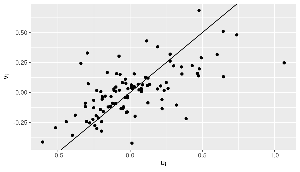
Figure 3.1: Posterior means of correlated random effects using a iid2d model. The solid line represents the identity line.

This type of correlated effects is commonly used in joint models, where different coefficients in the model need to be correlated. For example, in Chapter 12 a joint model is built to estimate height and weight. Because these two variables are usually highly correlated, their coefficients in regression models can sometimes be assumed to be similar.

3.3.9 Random walks (rw1 and rw2 models)

Random walks of order one and two are also available as latent effects in INLA. Given a vector of Gaussian observations \(u = (u_1,\ldots, u_n)\), the random walk of order one is defined assuming that increments \(\Delta u_i = u_{i} - u_{i-1}\) follow a Gaussian distribution with zero mean and precision \(\tau\). This is equivalent to assuming that the distribution of vector \(u\) is Gaussian with zero mean and precision matrix \(\tau Q\), where \(Q\) contains the neighborhood structure of the model.

Similarly, the random walk of order two is defined by assuming that second order increments \(\Delta^2 u_i = u_{i} - 2u_{i-1} + u_{i-2}\) follow a Gaussian distribution with zero mean and precision \(\tau\).

In both cases the random walk can be defined to be cyclic, and the model can be scaled to have an average variance (i.e., the diagonal of the generalized inverse of \(Q\)) equal to 1 (see Section 5.6). See Table 3.7 for options cyclic and scale.model, respectively.

Although this is a discrete latent effect, it can be used to model continuous variables by using the values argument. In particular, the values of the covariate can be binned so that they are associated with a particular value of the vector of random effects. This is particularly interesting to model non-linear dependence on covariates in the linear predictor.

A continuous random walk of order 2 is implemented as model crw2 in INLA. See Chapter 3 in Rue and Held (2005) for details on how this model is defined as a latent Gaussian Markov random field. In particular, these models are consistent with respect to the choice of the locations and the resolution, and their precision matrix is sparse due to the fact that they fulfill a Markov property.

Table 3.7: Summary of options of the rw1d and rw2d random effects.

Argument	Default	Description
values	—	Values of the covariate for which the effect is estimated.
cyclic	FALSE	Cyclic adjacency.
scale.model	FALSE	Whether to scale variance matrix.

The AirPassengers dataset records the number of total monthly international airline passengers from 1949 to 1960 (Box, Jenkins, and Reinsel 1976). This data is an object of class ts (i.e., time-series) and the next lines of R code show how to load the data and create a data.frame with the number of passengers, year, month of the year and id to identify the row in the dataset:

data(AirPassengers)

airp.data <- data.frame(airp = as.vector(AirPassengers),
  month = as.factor(rep(1:12, 12)), 
  year = as.factor(rep(1949:1960, each = 12)),
  ID = 1:length(AirPassengers))

Figure 3.2 shows the original times series and the log of the number of passengers. The original data show an increasing variance with time, which is not observed in the log-transformed time series. Given that the random walk assumes a common precision, it will be better to model the data in the log-scale.

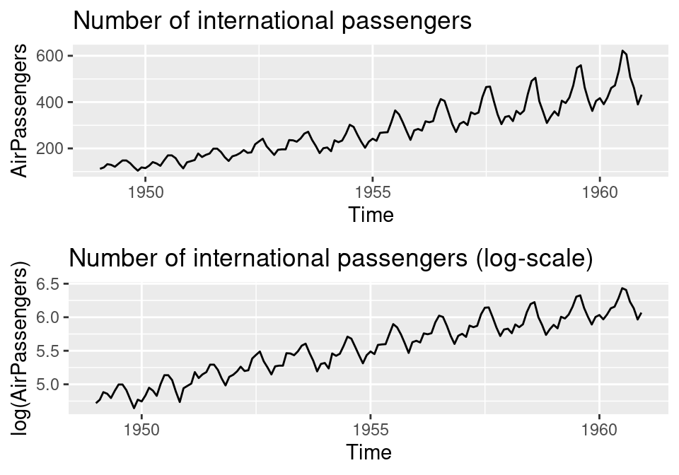
Figure 3.2: Monthly international airline passengers: original data (top) and log-scale (bottom).

The first model to be fit to the data is a linear model with a fixed effect on year and a rw1 random effect:

airp.rw1 <- inla(log(AirPassengers) ~ 0 + year + f(ID, model = "rw1"),
  control.family = list(hyper = list(prec = list(param = c(1, 0.2)))),
  data = airp.data, control.predictor = list(compute = TRUE))

summary(airp.rw1)

## 
## Call:
##    c("inla(formula = log(AirPassengers) ~ 0 + year + f(ID, model = 
##    \"rw1\"), ", " data = airp.data, control.predictor = list(compute 
##    = TRUE), ", " control.family = list(hyper = list(prec = list(param 
##    = c(1, ", " 0.2)))))") 
## Time used:
##     Pre = 0.328, Running = 0.573, Post = 0.112, Total = 1.01 
## Fixed effects:
##           mean    sd 0.025quant 0.5quant 0.975quant  mode kld
## year1949 5.157 0.252      4.664    5.156      5.654 5.154   0
## year1950 5.207 0.220      4.776    5.206      5.641 5.205   0
## year1951 5.332 0.190      4.959    5.332      5.707 5.331   0
## year1952 5.420 0.165      5.096    5.420      5.745 5.420   0
## year1953 5.490 0.146      5.203    5.490      5.776 5.490   0
## year1954 5.517 0.135      5.251    5.517      5.782 5.517   0
## year1955 5.602 0.135      5.335    5.602      5.867 5.603   0
## year1956 5.670 0.146      5.381    5.670      5.956 5.671   0
## year1957 5.727 0.165      5.401    5.728      6.051 5.729   0
## year1958 5.736 0.190      5.360    5.736      6.109 5.737   0
## year1959 5.806 0.219      5.374    5.807      6.237 5.807   0
## year1960 5.843 0.251      5.348    5.843      6.336 5.844   0
## 
## Random effects:
##   Name     Model
##     ID RW1 model
## 
## Model hyperparameters:
##                                           mean    sd 0.025quant 0.5quant
## Precision for the Gaussian observations 100.92 18.11      69.24    99.68
## Precision for ID                        157.70 42.63      93.83   150.91
##                                         0.975quant   mode
## Precision for the Gaussian observations     139.98  97.46
## Precision for ID                            259.68 138.00
## 
## Expected number of effective parameters(stdev): 58.90(8.78)
## Number of equivalent replicates : 2.44 
## 
## Marginal log-Likelihood:  2.04 
## Posterior marginals for the linear predictor and
##  the fitted values are computed

Next, a rw2 model is fitted:

airp.rw2 <- inla(log(AirPassengers) ~ 0 + year + f(ID, model = "rw2"),
  control.family = list(hyper = list(prec = list(param = c(1, 0.2)))),
  data = airp.data, control.predictor = list(compute = TRUE))
summary(airp.rw2)

## 
## Call:
##    c("inla(formula = log(AirPassengers) ~ 0 + year + f(ID, model = 
##    \"rw2\"), ", " data = airp.data, control.predictor = list(compute 
##    = TRUE), ", " control.family = list(hyper = list(prec = list(param 
##    = c(1, ", " 0.2)))))") 
## Time used:
##     Pre = 0.314, Running = 0.579, Post = 0.0333, Total = 0.927 
## Fixed effects:
##           mean    sd 0.025quant 0.5quant 0.975quant  mode kld
## year1949 5.148 0.278      4.602    5.148      5.694 5.148   0
## year1950 5.203 0.243      4.726    5.203      5.679 5.203   0
## year1951 5.323 0.210      4.909    5.323      5.736 5.323   0
## year1952 5.417 0.183      5.058    5.417      5.775 5.417   0
## year1953 5.467 0.162      5.149    5.467      5.784 5.467   0
## year1954 5.501 0.150      5.206    5.501      5.795 5.501   0
## year1955 5.585 0.149      5.291    5.585      5.879 5.585   0
## year1956 5.653 0.161      5.336    5.653      5.969 5.653   0
## year1957 5.715 0.182      5.357    5.715      6.073 5.715   0
## year1958 5.755 0.210      5.341    5.755      6.168 5.755   0
## year1959 5.847 0.243      5.369    5.847      6.325 5.847   0
## year1960 5.893 0.279      5.344    5.893      6.442 5.893   0
## 
## Random effects:
##   Name     Model
##     ID RW2 model
## 
## Model hyperparameters:
##                                           mean     sd 0.025quant 0.5quant
## Precision for the Gaussian observations 101.56  16.59      72.31   100.45
## Precision for ID                        409.79 138.21     208.67   386.27
##                                         0.975quant   mode
## Precision for the Gaussian observations     137.37  98.45
## Precision for ID                            745.52 343.97
## 
## Expected number of effective parameters(stdev): 47.16(4.53)
## Number of equivalent replicates : 3.05 
## 
## Marginal log-Likelihood:  -12.71 
## Posterior marginals for the linear predictor and
##  the fitted values are computed

Note that control.family has been used to set a prior on the precision of the Gaussian likelihood to prevent overfitting (J. J. Faraway 2019b; Bakka 2019). See also Chapter 5 on priors and Section 6.5.2.

In order to compare how these two models fit the data, the times series (in the log scale) and the fitted values from these two models have been plotted in Figure 3.3. In general, fitted values from both models are very close to the observed time series. However, the estimates obtained with the rw2 model seem to be smoother than those obtained with the rw1. This is not surprising as the rw2 is of a higher order.

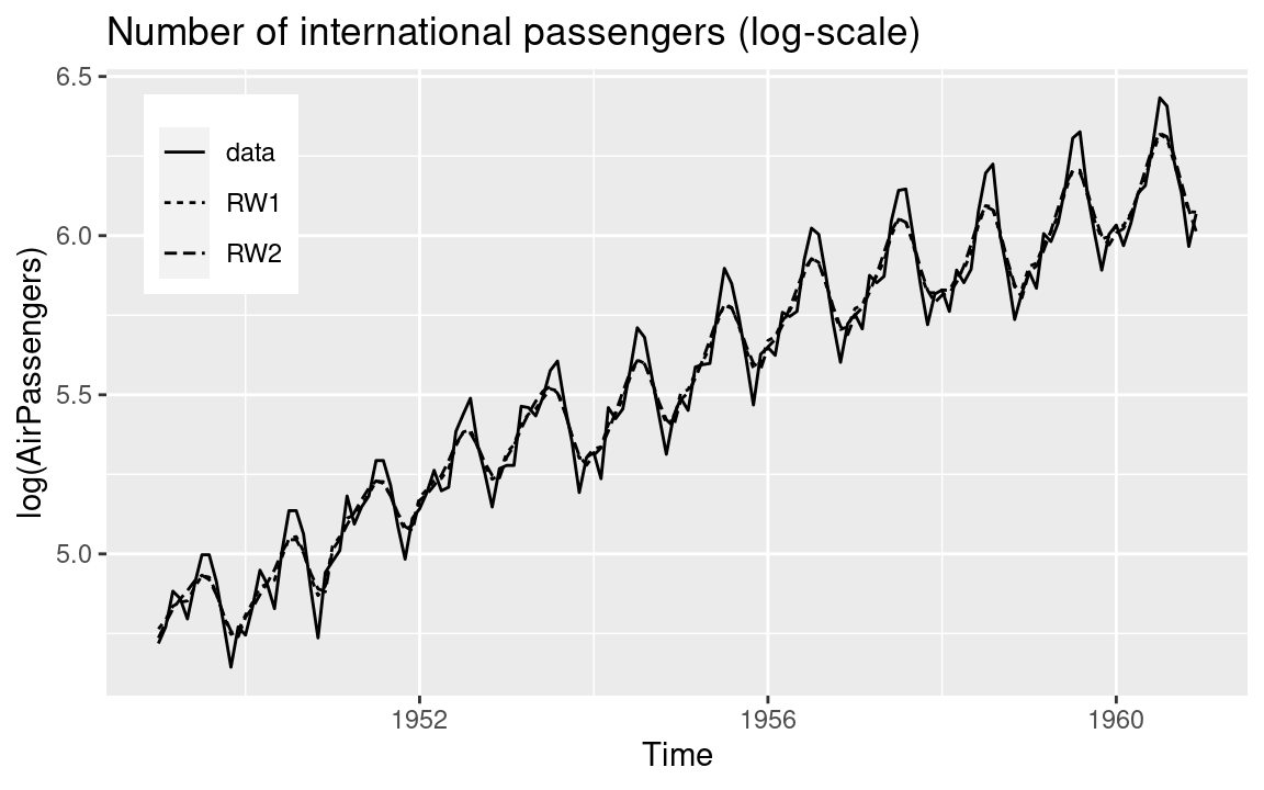
Figure 3.3: Fitted values (i.e., posterior means) of the number of international passengers.

Note that in this example, the latent effects are based on modeling the time series using values that are close in time, such as the one or two previous values. However, it is clear from Figure 3.2 that the time series has a strong season effect of period equal to one year. For this reason, it may be better to include a seasonal latent effect in the linear predictor.

3.3.10 Seasonal random effects

Seasonal effects can be modeled with the seasonal latent effect. In this case, the vector of random effects \(\mathbf{u} = (u_1,\ldots, u_n)\) is assumed to have periodicity \(p\) (with \(p < n\)) and it is defined such as sums \(x_i + x_{i+1} + \ldots + x_{i+m-1}\) are independent Gaussian observations with zero mean and precision \(\tau\).

Note that the precision matrix of the model is \(Q = \tau R\), where \(R\) has the neighborhood structure of the model. This model can be scaled, similarly to the random walk models. See Table 3.8 for the different specific options of this model. Note how periodicity of the seasonal effect can be set with argument season.length when the model is defined within the f() function.

For seasonal latent effects, the internal parameter is \(\theta = \log(\tau)\), and the default prior is a log-Gamma with parameters 1 and \(0.00005\). This prior can be modified as usual. See Section 3.5.1 and Chapter 5.

A seasonal model can be fit to the air passengers dataset as seen below. Note that we have set the periodicity to 12 so that the latent effect assumes that the seasonal effect covers one year. This is reasonable because the time series shows a clear seasonal effect of period equal to one year.

Table 3.8: Summary of options of the seasonal random effect.

Argument	Default	Description
season.length	—	Periodicity of the seasonal effect.
scale.model	FALSE	Whether to scale variance matrix.

Hence, the model is fit and summarized as follows:

airp.seasonal <- inla(log(AirPassengers) ~ 0 + year +
    f(ID, model = "seasonal", season.length = 12),
  control.family = list(hyper = list(prec = list(param = c(1, 0.2)))),
  data = airp.data)
summary(airp.seasonal)

## 
## Call:
##    c("inla(formula = log(AirPassengers) ~ 0 + year + f(ID, model = 
##    \"seasonal\", ", " season.length = 12), data = airp.data, 
##    control.family = list(hyper = list(prec = list(param = c(1, ", " 
##    0.2)))))") 
## Time used:
##     Pre = 0.321, Running = 0.383, Post = 0.0281, Total = 0.732 
## Fixed effects:
##           mean   sd 0.025quant 0.5quant 0.975quant  mode kld
## year1949 4.836 0.02      4.797    4.836      4.875 4.836   0
## year1950 4.931 0.02      4.891    4.931      4.970 4.931   0
## year1951 5.131 0.02      5.092    5.131      5.171 5.131   0
## year1952 5.277 0.02      5.238    5.277      5.317 5.277   0
## year1953 5.409 0.02      5.369    5.409      5.448 5.409   0
## year1954 5.467 0.02      5.427    5.467      5.506 5.467   0
## year1955 5.639 0.02      5.600    5.639      5.679 5.639   0
## year1956 5.784 0.02      5.745    5.784      5.824 5.784   0
## year1957 5.898 0.02      5.859    5.898      5.938 5.898   0
## year1958 5.931 0.02      5.891    5.931      5.970 5.931   0
## year1959 6.048 0.02      6.009    6.048      6.088 6.048   0
## year1960 6.154 0.02      6.115    6.154      6.194 6.154   0
## 
## Random effects:
##   Name     Model
##     ID Seasonal model
## 
## Model hyperparameters:
##                                             mean       sd 0.025quant
## Precision for the Gaussian observations   212.37    27.41     162.69
## Precision for ID                        40021.83 24480.36   10396.94
##                                         0.5quant 0.975quant     mode
## Precision for the Gaussian observations   211.00     270.28   208.66
## Precision for ID                        34433.18  103017.17 24596.27
## 
## Expected number of effective parameters(stdev): 26.52(1.85)
## Number of equivalent replicates : 5.43 
## 
## Marginal log-Likelihood:  70.22

3.3.11 Autoregressive random effects

Autoregressive models of order \(p\), denoted by AR(\(p\)), are also available in INLA. In particular, an autoregressive model of order 1 (ar1) and a generic order \(p\) (ar) are implemented.

The AR(1) model on a vector \(\mathbf{u}\) can be defined as \(u_1\) coming from a Gaussian distribution with zero mean and precision \(\tau (1 -\rho^2)\), where \(\tau\) is a precision parameter and \(\rho\) a correlation coefficient so that \(|\rho| < 1\). The other elements in \(\mathbf{u}\) are defined as \(u_i = \rho x_{i-1} + \varepsilon_i, i=2,\ldots,n\) with \(\varepsilon\) Gaussian observation with zero mean and precision \(\tau\).

Similarly as for the random walk models, autoregressive models can take the values argument when defined to set the values of the covariates for which the effects are being estimated. For the ar1 model, covariates can be included using argument control.ar1c when defining the model. Table 3.9 summarizes the specific options of the autoregressive latent effects.

Table 3.9: Summary of options of the ar1, ar1c and ar random effects.

Argument	Default	Description
values	—	Values of the covariate for which the effect is estimated.
order	—	Order of autoregressive model (for ar only).
control.ar1c	—	List with two objects: Z and Q.beta.
control.ar1c$Z	—	Matrix of covariates of dimension \(n\times m\).
control.ar1c$Q.beta	—	\(m\times m\) precision matrix of Gaussian prior on the coefficients of the covariates.

This model is parameterized using \(\bm\theta = (\theta_1, \theta_2)\). The first internal hyperparameter is defined as \(\theta_1 = \log(\kappa)\), where \(\kappa\) is the marginal precision:

\[ \kappa = \tau (1 - \rho^2) \]

The second hyperparameter is defined as

\[ \theta_2 = \log(\frac{1 + \rho}{1 - \rho}) \]

The prior is defined on \(\theta\). The default is a log-Gamma with parameters \(1\) and \(0.00005\) for \(\theta_1\) and a Gaussian with zero mean and precision 1 for \(\theta_2\).

The AR(1) model can be extended to include covariates as follows:

\[ u_i = \rho u_{i-1} + \sum_{j=1}^m \beta_j z_{i-1}^{(j)}+\varepsilon_i, i=2,\ldots,n \]

This model is known as ar1c. Here, \(m\) covariates are used in the model, and \(z_{i}^{(j)}\) is the value of the covariate \(j\) of observation \(i\). The covariates have associated coefficients \(\beta_j, j=1,\ldots,m\).

Coefficients are assigned a multivariate Gaussian prior with known precision matrix. The matrix of covariates (by column) and the precision of the prior on the coefficients are defined in the f() function via parameter control.ar1c, and they are passed as a list with names Z and Q.beta, respectively. See Table 3.9 for details.

The AR(p) model is defined in a similar way, but it can now include a lag of order \(p\) on the vector of random effects:

\[ u_i = \varphi_1 x_{i-1} + \ldots + \varphi_p u_{i-p} + \varepsilon_i, i = p,\ldots, n \]

Note that this model can handle values of \(p\) up to 10 (inclusive). The internal parameterization of this model is more complex and we refer the reader to the manual page, which can be accessed with inla.doc("^ar$"). The argument of inla.doc is due to the fact that this function used regular expressions to look up in the documentation files.

To illustrate the use of autoregressive models with INLA we will fit a number of models to the AirPassengers dataset. We will start with an AR(1) model:

airp.ar1 <- inla(log(AirPassengers) ~ 0 + year + f(ID, model = "ar1"),
  control.family = list(hyper = list(prec = list(param = c(1, 0.2)))),
  data = airp.data, control.predictor = list(compute = TRUE))
summary(airp.ar1)

## 
## Call:
##    c("inla(formula = log(AirPassengers) ~ 0 + year + f(ID, model = 
##    \"ar1\"), ", " data = airp.data, control.predictor = list(compute 
##    = TRUE), ", " control.family = list(hyper = list(prec = list(param 
##    = c(1, ", " 0.2)))))") 
## Time used:
##     Pre = 0.328, Running = 0.203, Post = 0.0352, Total = 0.566 
## Fixed effects:
##           mean    sd 0.025quant 0.5quant 0.975quant  mode kld
## year1949 4.843 0.084      4.679    4.842      5.016 4.840   0
## year1950 4.940 0.081      4.782    4.939      5.104 4.938   0
## year1951 5.129 0.080      4.969    5.129      5.289 5.129   0
## year1952 5.277 0.080      5.117    5.277      5.436 5.277   0
## year1953 5.403 0.080      5.242    5.403      5.562 5.403   0
## year1954 5.478 0.080      5.320    5.477      5.640 5.476   0
## year1955 5.638 0.080      5.478    5.638      5.797 5.638   0
## year1956 5.776 0.080      5.614    5.777      5.934 5.778   0
## year1957 5.888 0.081      5.725    5.889      6.045 5.890   0
## year1958 5.932 0.080      5.771    5.933      6.091 5.933   0
## year1959 6.046 0.081      5.883    6.047      6.205 6.048   0
## year1960 6.124 0.085      5.948    6.127      6.287 6.130   0
## 
## Random effects:
##   Name     Model
##     ID AR1 model
## 
## Model hyperparameters:
##                                            mean     sd 0.025quant 0.5quant
## Precision for the Gaussian observations 102.202 18.159     70.452  100.929
## Precision for ID                         63.951 21.353     29.925   61.540
## Rho for ID                                0.752  0.074      0.591    0.758
##                                         0.975quant   mode
## Precision for the Gaussian observations    141.470 98.625
## Precision for ID                           112.634 56.536
## Rho for ID                                   0.879  0.769
## 
## Expected number of effective parameters(stdev): 62.15(8.37)
## Number of equivalent replicates : 2.32 
## 
## Marginal log-Likelihood:  4.69 
## Posterior marginals for the linear predictor and
##  the fitted values are computed

Next, an AR(3) is fitted:

airp.ar3 <- inla(log(AirPassengers) ~ 0 + year + f(ID, model = "ar",
    order = 3), 
  control.family = list(hyper = list(prec = list(param = c(1, 0.2)))),
  data = airp.data, control.predictor = list(compute = TRUE))
summary(airp.ar3)

## 
## Call:
##    c("inla(formula = log(AirPassengers) ~ 0 + year + f(ID, model = 
##    \"ar\", ", " order = 3), data = airp.data, control.predictor = 
##    list(compute = TRUE), ", " control.family = list(hyper = list(prec 
##    = list(param = c(1, ", " 0.2)))))") 
## Time used:
##     Pre = 0.332, Running = 0.563, Post = 0.0471, Total = 0.942 
## Fixed effects:
##           mean    sd 0.025quant 0.5quant 0.975quant  mode kld
## year1949 4.835 0.027      4.782    4.835      4.888 4.835   0
## year1950 4.930 0.027      4.877    4.930      4.983 4.930   0
## year1951 5.131 0.027      5.078    5.131      5.184 5.131   0
## year1952 5.277 0.027      5.225    5.277      5.330 5.277   0
## year1953 5.408 0.027      5.355    5.408      5.460 5.408   0
## year1954 5.465 0.027      5.412    5.465      5.518 5.465   0
## year1955 5.639 0.027      5.586    5.639      5.691 5.639   0
## year1956 5.784 0.027      5.731    5.784      5.837 5.784   0
## year1957 5.898 0.027      5.845    5.898      5.950 5.898   0
## year1958 5.930 0.027      5.877    5.930      5.983 5.930   0
## year1959 6.048 0.027      5.995    6.048      6.101 6.048   0
## year1960 6.154 0.027      6.101    6.154      6.207 6.154   0
## 
## Random effects:
##   Name     Model
##     ID AR(p) model
## 
## Model hyperparameters:
##                                            mean     sd 0.025quant 0.5quant
## Precision for the Gaussian observations 122.636 12.136     99.027  122.679
## Precision for ID                        181.637 94.418     55.927  163.237
## PACF1 for ID                              0.849  0.004      0.841    0.848
## PACF2 for ID                             -0.757  0.045     -0.845   -0.756
## PACF3 for ID                             -0.948  0.013     -0.967   -0.951
##                                         0.975quant    mode
## Precision for the Gaussian observations    146.707 123.526
## Precision for ID                           417.007 127.378
## PACF1 for ID                                 0.859   0.847
## PACF2 for ID                                -0.663  -0.750
## PACF3 for ID                                -0.914  -0.956
## 
## Expected number of effective parameters(stdev): 20.51(1.46)
## Number of equivalent replicates : 7.02 
## 
## Marginal log-Likelihood:  39.40 
## Posterior marginals for the linear predictor and
##  the fitted values are computed

In previous models covariate year has been included as part of the linear predictor. In the next model this covariate is included as part of an AR(1) model with covariates (i.e., a ar1c model):

Z <- model.matrix (~ 0 + year, data = airp.data)
Q.beta <- Diagonal(12, 0.001)

airp.ar1c <- inla(log(AirPassengers) ~ 1 + f(ID, model = "ar1c",
  args.ar1c = list(Z = Z, Q.beta = Q.beta)),
  control.family = list(hyper = list(prec = list(param = c(1, 0.2)))),
  data = airp.data, control.predictor = list(compute = TRUE))
summary(airp.ar1c)

## 
## Call:
##    c("inla(formula = log(AirPassengers) ~ 1 + f(ID, model = \"ar1c\", 
##    ", " args.ar1c = list(Z = Z, Q.beta = Q.beta)), data = airp.data, 
##    ", " control.predictor = list(compute = TRUE), control.family = 
##    list(hyper = list(prec = list(param = c(1, ", " 0.2)))))") 
## Time used:
##     Pre = 0.214, Running = 0.266, Post = 0.0362, Total = 0.516 
## Fixed effects:
##              mean    sd 0.025quant 0.5quant 0.975quant  mode kld
## (Intercept) 4.724 0.135      4.458    4.724       4.99 4.724   0
## 
## Random effects:
##   Name     Model
##     ID AR1C model
## 
## Model hyperparameters:
##                                            mean     sd 0.025quant 0.5quant
## Precision for the Gaussian observations  99.123 18.856     66.588   97.652
## Precision for ID                        119.087 36.651     64.630  113.167
## Rho for ID                                0.522  0.089      0.331    0.529
##                                         0.975quant    mode
## Precision for the Gaussian observations    140.425  94.936
## Precision for ID                           206.937 102.315
## Rho for ID                                   0.677   0.544
## 
## Expected number of effective parameters(stdev): 60.32(9.96)
## Number of equivalent replicates : 2.39 
## 
## Marginal log-Likelihood:  3.65 
## Posterior marginals for the linear predictor and
##  the fitted values are computed

In all three models, the autoregressive effect seems to capture the high temporal autocorrelation in the data given the estimates of the autocorrelation parameter. Figure 3.4 shows the original time series (in the log scale) together with the posterior means of the fitted values.

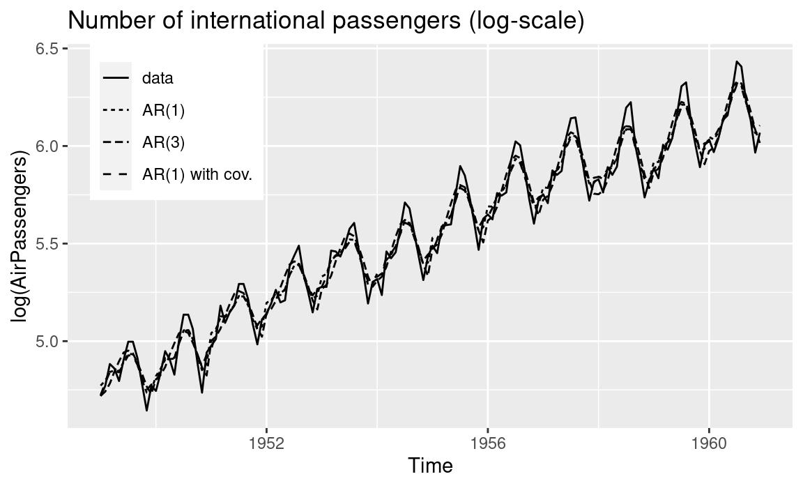
Figure 3.4: Fitted values (i.e., posterior means) of the number of international passengers using autoregressive models.

3.4 Information on the latent effects

The names of the hyperparameters in a given model, their internal parameterization and the default prior on the internal scale can be checked in the manual page (i.e., calling inla.doc()) or using function inla.models(). For example, the information about the idd model can be displayed with inla.models()$latent$iid, and similarly for any other random effects model.

This is particularly useful when in doubt about how a particular part of the model is defined, such as the internal representation of the parameters and their default priors. The full list of the elements that define the latent effect can be seen here:

names(inla.models()$latent$iid)

##  [1] "doc"                "hyper"              "constr"            
##  [4] "nrow.ncol"          "augmented"          "aug.factor"        
##  [7] "aug.constr"         "n.div.by"           "n.required"        
## [10] "set.default.values" "pdf"

Although particular random effects may require the use of specific parameters, there are a number of common parameters to all models that are worth knowing. These are described in the next section.

3.5 Additional arguments

In addition to the specific parameters required by each one of the random effects previously described, there are a number of other arguments that can be used to tune specific parts of the model. Some of these are summarized in Table 3.10. All of them must be passed to the f() function when defining the latent effect in the model formula.

Table 3.10: Summary of additional arguments that can be passed when defining a random effect.

Argument	Default	Description
hyper	Default priors	Definition of priors for hyperparameters.
constr	FALSE	Sum-to-zero constraint on the random effects.
extraconstr	FALSE	Additional constraint on the random effects.
scale.model	FALSE	Scale variance matrix of random effects.
group	—	Variable to define the groups of random effect.
control.group	—	Control options for group parameter.

3.5.1 Priors of hyperparameters

Priors in INLA are described in detail in Chapter 5 but we include here a short introduction to how priors are set. Priors on the model hyperparameters are set with parameter hyper, which takes a named list using the names of the hyperparameters. Each element in the named list must be one of the variables shown in Table 3.11.

For example, the default parameters for the prior on the log-precision of the random effects of a iid random effects are:

prec.prior <- inla.models()$latent$iid$hyper$theta
prec.prior

## $hyperid
## [1] 1001
## attr(,"inla.read.only")
## [1] FALSE
## 
## $name
## [1] "log precision"
## attr(,"inla.read.only")
## [1] FALSE
## 
## $short.name
## [1] "prec"
## attr(,"inla.read.only")
## [1] FALSE
## 
## $prior
## [1] "loggamma"
## attr(,"inla.read.only")
## [1] FALSE
## 
## $param
## [1] 1e+00 5e-05
## attr(,"inla.read.only")
## [1] FALSE
## 
## $initial
## [1] 4
## attr(,"inla.read.only")
## [1] FALSE
## 
## $fixed
## [1] FALSE
## attr(,"inla.read.only")
## [1] FALSE
## 
## $to.theta
## function (x) 
## log(x)
## <bytecode: 0x55a61a4dc528>
## <environment: 0x55a61a4d4c60>
## attr(,"inla.read.only")
## [1] TRUE
## 
## $from.theta
## function (x) 
## exp(x)
## <bytecode: 0x55a61a4dc640>
## <environment: 0x55a61a4d4c60>
## attr(,"inla.read.only")
## [1] TRUE

Note that in this case there is a single hyperparameter \(\theta\) and hence the $theta after hyper. Other random effects with more than one hyperparameter will name them theta1, etc.

In this example, the internal parameterization is \(\theta = \log(\tau)\) (prec.prior$to.theta above), with \(\tau\) the precision of the iid random effects. The default prior, on \(\theta\), is a log-Gamma (prec.prior$prior) with parameters \(1\) and \(0.00005\) (prec.prior$param), as seen in parameters prior and param. The starting value of \(\theta\) is \(4\), as seen in parameter prec.prior$initial and it is not fixed by default (i.e., a posterior marginal will be estimated) because prec.prior$fixed is FALSE. When fixed is set to TRUE, the hyperparameter will be kept constant at the value in initial. In this particular case, as initial is 4 this will make the log-precision to be \(4\), i.e., \(4 = \theta = \log(\tau)\), which implies that the precision would be fixed to \(\tau = \exp(4)\). This will represent a very large precision or, equivalently, a very small variance which will make the random effects very close to zero.

Furthermore, functions set in to.theta and from.theta are used to convert the values of \(\tau\) to and from \(\theta\) (i.e., from the model scale to and from the internal scale). In this case, given that \(\theta = \log(\tau)\), to.theta is the log() function while from.theta is the exp() function, because \(\tau = \exp(\theta)\).

Table 3.11: Summary of parameters that are used to define a prior on a hyperparameter with INLA.

Argument	Description
hyperid	Internal id of prior.
name	Name of hyperparameter in internal scale.
short.name	Short name of hyperparameter to be used inside hyper.
prior	Name of prior distribution.
param	Parameter values of prior distributions.
initial	Initial value of hyperparameter in the internal scale.
fixed	Whether to keep the hyperparameter fixed (default is FALSE).
to.theta	Function to convert parameter into the internal scale.
from.theta	Function to convert the value in the internal scale to the model scale.

In general, not all arguments in the prior definition will be given a value when setting a non-default prior. For example, in the iid model the prior on the log-precision could be replaced by a Gaussian with zero mean and small precision. This could be easily done as follows:

hyper = list(prec = list(prior = "gaussian", param = c(0, 0.001)))

The former R code sets a Gaussian prior with zero mean and precision \(0.001\) on \(\theta\), i.e., a log-Gaussian prior on \(\tau\).

A full example on the North Carolina SIDS data using this prior would be:

m.pois.iid.gp <- inla(SID74 ~ f(ID, model = "iid",
    hyper = list(theta = list(prior = "gaussian", param = c(0, 0.001)))),
  data = nc.sids, family = "poisson",
  E = EXP74)
summary(m.pois.iid.gp)

## 
## Call:
##    c("inla(formula = SID74 ~ f(ID, model = \"iid\", hyper = 
##    list(theta = list(prior = \"gaussian\", ", " param = c(0, 
##    0.001)))), family = \"poisson\", data = nc.sids, ", " E = EXP74)") 
## Time used:
##     Pre = 0.218, Running = 0.103, Post = 0.0183, Total = 0.339 
## Fixed effects:
##               mean    sd 0.025quant 0.5quant 0.975quant   mode kld
## (Intercept) -0.032 0.064     -0.162   -0.031      0.091 -0.028   0
## 
## Random effects:
##   Name     Model
##     ID IID model
## 
## Model hyperparameters:
##                  mean   sd 0.025quant 0.5quant 0.975quant mode
## Precision for ID 6.52 2.15       3.49     6.14      11.82 5.52
## 
## Expected number of effective parameters(stdev): 42.43(6.26)
## Number of equivalent replicates : 2.36 
## 
## Marginal log-Likelihood:  -241.89

The estimates of the parameters are very similar to the previous examples but not equal and this is due to the choice of the priors. Note that in the named list passed to hyper we have used prec to set the prior for the hyperparameter. An alternative name could have been theta. i.e.,

hyper = list(theta = list(prior = "gaussian", param = c(0, 0.001)))

However, using prec makes the code easier to read and avoids possible errors when setting the priors for models with several hyperparameters. In this case, the list passed to hyper can have length higher than one. For example, for a model with two hyperparameters this would be:

hyper = list(theta1 = list(...), theta2 = list(...))

Detailed information on how priors can be set in INLA (including implementing new priors and other features) is given in Chapter 5.

3.5.2 Sum-to-zero constraint

Some of the models described above are intrinsic, i.e., their precision matrices are singular. Hence, the distribution is improper and may lead to an improper posterior. In other words, the precision matrix is not full-rank and additional constraints on the random effects are often imposed (see also Section 6.3).

A common one is a sum-to-zero constraint which will make the values of the random effects \(\mathbf{u} = (u_1,\ldots, u_n)\) to be such as \(\sum_{i=1}^n u_i =0\). This can be achieved by setting parameter constr to TRUE when the model is defined. This sum-to-zero constraint is added by default to all intrinsic models implemented in INLA.

For example, for a rw1 model the constr parameter is set to TRUE by default:

inla.models()$latent$rw1$constr

## [1] TRUE

On the other hand, iid latent effects are not intrinsic and the parameter is set to FALSE by default:

inla.models()$latent$iid$constr

## [1] FALSE

Note that setting constraints on the random effects will likely affect the estimates of other parameters in the model as these constraints will shift the estimates of the random effects.

In the previous example on the North Carolina SIDS data, the way to add a sum-to-zero constraint on the iid random effects (using the default prior) would be:

m.pois.iid.gp0 <- inla(SID74 ~ f(ID, model = "iid", constr = TRUE),
  data = nc.sids, family = "poisson", E = EXP74)

summary(m.pois.iid.gp0)

## 
## Call:
##    c("inla(formula = SID74 ~ f(ID, model = \"iid\", constr = TRUE), 
##    family = \"poisson\", ", " data = nc.sids, E = EXP74)") 
## Time used:
##     Pre = 0.213, Running = 0.15, Post = 0.0182, Total = 0.381 
## Fixed effects:
##               mean    sd 0.025quant 0.5quant 0.975quant   mode kld
## (Intercept) -0.027 0.049     -0.126   -0.026      0.067 -0.025   0
## 
## Random effects:
##   Name     Model
##     ID IID model
## 
## Model hyperparameters:
##                  mean   sd 0.025quant 0.5quant 0.975quant mode
## Precision for ID 7.26 2.57       3.79     6.77      13.61 6.02
## 
## Expected number of effective parameters(stdev): 40.44(6.52)
## Number of equivalent replicates : 2.47 
## 
## Marginal log-Likelihood:  -245.54

In this particular case, the parameter estimates are quite similar.

3.5.3 Additional constraints on the random effects

In addition to the sum-to-zero constraint there is also the possibility of setting additional constraints on the random effects. See Section 6.3 for a general discussion on how to set linear constraints on the latent effects in INLA.

Linear constraints are set with argument extraconstr. This will take a list with two elements, A and e, to define the constraint \(A \mathbf{u} = e\). Hence, A must be a matrix with the same number of columns as the length of the vector of random effects, and e must be a vector of the appropriate length, i.e., with the same number of rows as matrix A.

For example, a sum-to-zero constraint for a vector of random effects of length n could be added as follows:

A <- matrix(1, ncol = n, nrow = 1)
e <- rep(0, 1)

inla( ... ~ ... + f(..., extraconstr = list(A, e), ...), ...)

Hence, the previous example could be reproduced as follows using extraconstr:

n <- nrow(nc.sids)
A <- matrix(1, ncol = n, nrow = 1)
e <- rep(0, 1)
m.pois.iid.extrac <- inla(SID74 ~ 
    f(ID, model = "iid", extraconstr = list(A = A, e = e)),
  data = nc.sids, family = "poisson", E = EXP74)

summary(m.pois.iid.extrac)

## 
## Call:
##    c("inla(formula = SID74 ~ f(ID, model = \"iid\", extraconstr = 
##    list(A = A, ", " e = e)), family = \"poisson\", data = nc.sids, E 
##    = EXP74)" ) 
## Time used:
##     Pre = 0.223, Running = 0.146, Post = 0.0189, Total = 0.388 
## Fixed effects:
##               mean    sd 0.025quant 0.5quant 0.975quant   mode kld
## (Intercept) -0.027 0.049     -0.126   -0.026      0.067 -0.025   0
## 
## Random effects:
##   Name     Model
##     ID IID model
## 
## Model hyperparameters:
##                  mean   sd 0.025quant 0.5quant 0.975quant mode
## Precision for ID 7.26 2.57       3.79     6.77      13.61 6.02
## 
## Expected number of effective parameters(stdev): 40.44(6.52)
## Number of equivalent replicates : 2.47 
## 
## Marginal log-Likelihood:  -245.54

Note how the fit model is the same as the previous one.

The main purpose to add additional constraint is for identifiability purposes. See, for example, Rue and Held (2005) for more details on this topic. Goicoa et al. (2018) show how additional constraints on the random effect can change the model estimates in spatio-temporal disease mapping models. However, this behavior is likely to be reproduced by models where the random effects are highly constrained for identifiability reasons.

3.5.4 Model scaling

Another feature that is particularly interesting when dealing with intrinsic models is the possibility to scale the model to make the diagonal of the structure variance (i.e., excluding the precision parameter) of the random effects to be re-scaled so that the generalized variance is equal to 1. This is fully described in Sørbye and Rue (2014), with a more practical example available in Sørbye (2013). Scaling in the context of prior setting is discussed later in Section 5.6.

The generalized variance is the geometric mean of the diagonal values of the covariance matrix (see Sørbye 2013 for details). By setting this to one the precision parameter is re-scaled as well. As a result of this scaling, the precision parameters of different models will have a similar interpretation. Hence, imposing the same priors on them (e.g., the default prior) will make sense as they are in the same scale. Furthermore, scaled models will be less sensible to the scale of the data used to estimate the effects (as shown in Sørbye 2013).

Scaling is set with parameter scale.model, which is FALSE by default. The rw1 model fit to the air passengers data can be modified to scale the latent random effect:

airp.rw1.scale <- inla(log(AirPassengers) ~ 0 + year +
    f(ID, model = "rw1", scale.model = TRUE),
  control.family = list(hyper = list(prec = list(param = c(1, 0.2)))),
  data = airp.data)

summary(airp.rw1.scale)

## 
## Call:
##    c("inla(formula = log(AirPassengers) ~ 0 + year + f(ID, model = 
##    \"rw1\", ", " scale.model = TRUE), data = airp.data, 
##    control.family = list(hyper = list(prec = list(param = c(1, ", " 
##    0.2)))))") 
## Time used:
##     Pre = 0.313, Running = 0.377, Post = 0.0284, Total = 0.718 
## Fixed effects:
##           mean    sd 0.025quant 0.5quant 0.975quant  mode kld
## year1949 5.157 0.252      4.664    5.156      5.654 5.154   0
## year1950 5.207 0.220      4.776    5.206      5.641 5.205   0
## year1951 5.332 0.190      4.959    5.332      5.707 5.331   0
## year1952 5.420 0.165      5.096    5.420      5.745 5.420   0
## year1953 5.490 0.146      5.203    5.490      5.776 5.490   0
## year1954 5.517 0.135      5.251    5.517      5.782 5.517   0
## year1955 5.602 0.135      5.335    5.602      5.867 5.603   0
## year1956 5.670 0.146      5.382    5.670      5.956 5.671   0
## year1957 5.727 0.165      5.401    5.728      6.051 5.729   0
## year1958 5.736 0.190      5.360    5.736      6.109 5.737   0
## year1959 5.806 0.219      5.374    5.807      6.237 5.807   0
## year1960 5.843 0.251      5.348    5.843      6.335 5.844   0
## 
## Random effects:
##   Name     Model
##     ID RW1 model
## 
## Model hyperparameters:
##                                           mean    sd 0.025quant 0.5quant
## Precision for the Gaussian observations 100.81 18.10      69.21    99.54
## Precision for ID                          7.25  1.96       4.31     6.93
##                                         0.975quant  mode
## Precision for the Gaussian observations     139.99 97.24
## Precision for ID                             11.94  6.34
## 
## Expected number of effective parameters(stdev): 58.89(8.79)
## Number of equivalent replicates : 2.44 
## 
## Marginal log-Likelihood:  -221.27

Figure 3.5 shows the effect of scaling a rw1 model. The point estimates of the random effects do not seem to change but the posterior marginals of the precision are clearly in different scales. Note that this also means that the linear predictor is not affected by re-scaling and the fitted values will be the same. For the scaled model, the posterior marginal show smaller values than the one obtained with the non-scaled model.

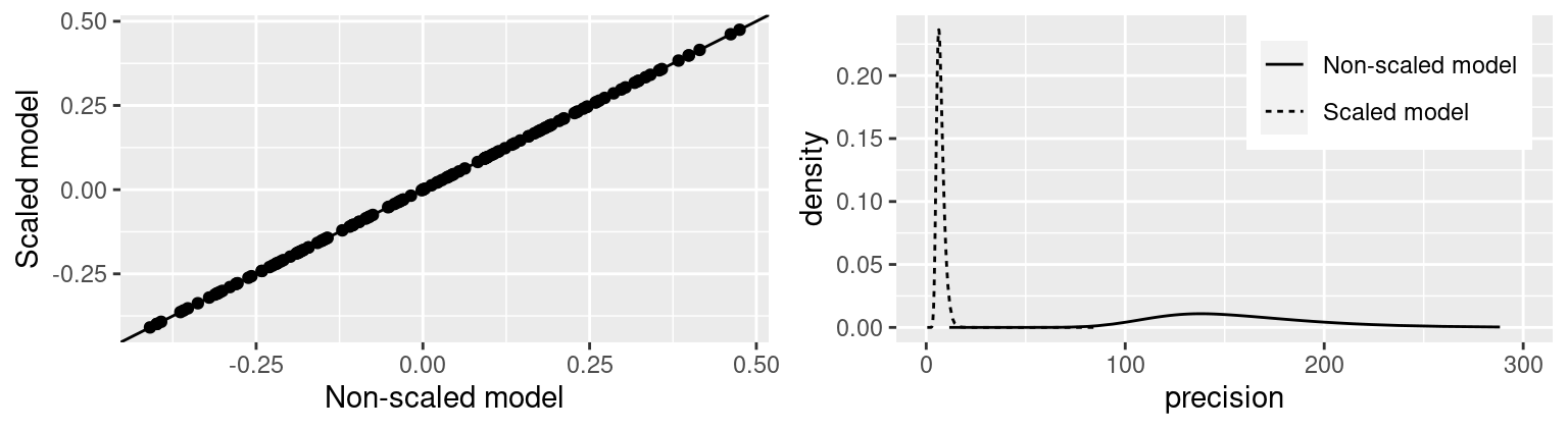
Figure 3.5: Non-scaled versus scaled models. Point estimates (i.e., posterior means) of the random effects (left) and posterior marginal of the precision of the random effect (right).

3.5.5 Grouped effects

Random effects can be grouped so that additional group-level correlation can be included using an appropriate latent effect. The variable that sets the group must be passed with parameter group and the actual model and other parameters are passed through the control.group parameter. This adds a new model to account for between group correlation, i.e., observations are already correlated using the primary random effects but also according to the grouped effect. In practice, the variance structure of the resulting model is the Kronecker product of the main and grouped random effects. This is further discussed in Section 8.6, where spatio-temporal models are discussed.

Table 3.12: Summary of options to be set with control.group when defining grouped random effects.

Argument	Description
adjust.for.con.comp	Adjust for connected components when the model is scaled (default is TRUE).
cyclic	Make the group model cyclic (only for ar1, rw1 and rw2 models)
graph	Graph specification (for besag model).
hyper	Definition of priors in the hyperparameters.
model	Group model (exchangable, exchangablepos, ar1, ar, rw1, rw2, besag or iid).
order	Order of the model (only available for ar models).
scale.model	Scale the grouped model (default is TRUE; only for rw1, rw2 or besag models).

Table 3.12 shows a summary of the options that can be passed to control.group. In general, these are the same that apply to the random effect when it is used.

In the next example we will analyze the air passengers data by using iid random effects on the year but correlated random effects using an ar1 model for the months. This implies that the observations for the same month of consecutive years are correlated. First of all, two integer indices from 1 to 12 are created for the month (particularly important as this is passed to group) and year, and then the model is fitted:

airp.data$month.num <- as.numeric(airp.data$month)
airp.data$year.num <- as.numeric(airp.data$year)
airp.iid.ar1 <- inla(log(airp) ~ 0 +  f(year.num, model = "iid",
    group = month.num, control.group = list(model = "ar1", 
    scale.model = TRUE)),
  data = airp.data)
summary(airp.iid.ar1)

## 
## Call:
##    c("inla(formula = log(airp) ~ 0 + f(year.num, model = \"iid\", 
##    group = month.num, ", " control.group = list(model = \"ar1\", 
##    scale.model = TRUE)), ", " data = airp.data)") 
## Time used:
##     Pre = 0.215, Running = 0.195, Post = 0.0218, Total = 0.432 
## Random effects:
##   Name     Model
##     year.num IID model
## 
## Model hyperparameters:
##                                             mean       sd 0.025quant
## Precision for the Gaussian observations 2.22e+04 2.05e+04   2476.378
## Precision for year.num                  4.70e-02 1.60e-02      0.022
## GroupRho for year.num                   1.00e+00 0.00e+00      0.999
##                                         0.5quant 0.975quant    mode
## Precision for the Gaussian observations 1.65e+04   7.64e+04 6969.55
## Precision for year.num                  4.40e-02   8.40e-02    0.04
## GroupRho for year.num                   1.00e+00   1.00e+00    1.00
## 
## Expected number of effective parameters(stdev): 142.40(1.67)
## Number of equivalent replicates : 1.01 
## 
## Marginal log-Likelihood:  43.34

Figure 3.6 shows the posterior estimates of the grouped random effects. Each plot represents a given month, and the increasing trend is clearly visible. In the model summary this can be appreciated by looking at the high correlation of the grouped effect, which has a posterior mean of 0.9997. Note also how summer months, for example, have higher estimates of the number of passengers.

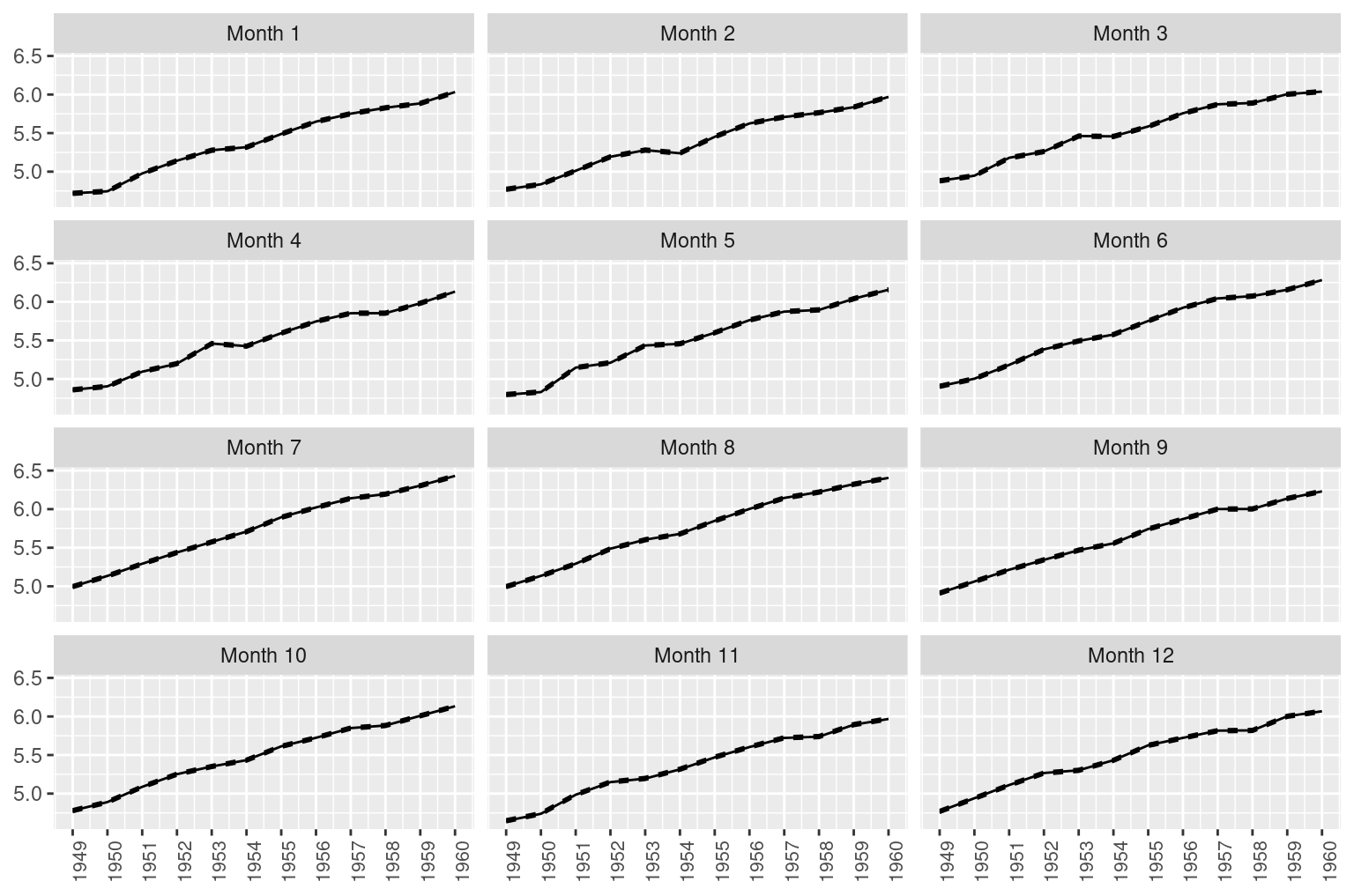
Figure 3.6: Grouped effects for the air passengers dataset. Solid lines represent the posterior means and the dashed lines 95% credible intervals.

3.6 Final remarks

In this chapter we have described some of the random effects implemented in the INLA package. However, this list is far from exhaustive. Table 3.13 shows a list of other random effects not discussed in this chapter. As INLA keeps growing, the list of available latent effects is likely to increase too, so the list below may miss some recent developments. Spatial random effects are described in detail in Chapter 7. In general, detailed information about the random effects can be obtained from the manual page that can be accessed with function inla.doc(). This function takes the name of the latent effect to be searched, e.g., inla.doc("ou").

Table 3.13: Summary of other random effects not described in this chapter.

Model	Description
ou	Ornstein-Uhlenbeck process.
sigm	Sigmoidal effect of a covariate.
revsigm	Reverse-sigmoidal effect of a covariate.
mec	Classical measurement error model.
meb	Berkson Measurement Error model.
matern2d	Gaussian field with Matérn correlation in a 2D lattice.
rw2d	2-dimensional random walk.
besag	Besag spatial model.
besag2	Weighted spatial effects model.
besagproper	Convolution spatial model.
besagproper2	Convolution spatial model.
bym	Convolution spatial model.
bym2	Reparameterized convolution spatial model.
slm	Spatial lag model.
spde	Spatial model based on Stochastic Partial Differential Equations.
rgeneric	Generic random effect.
fgn	Fractional Gaussian noise.
fgn2	Reparameterized fractional Gaussian noise.
copy	Copy a random effect.
log1exp	Non-linear effect of a positive covariate.
logdist	Non-linear effect of a positive covariate.

References

Bakka, Haakon. 2019. “Small Tutorials on INLA.” https://haakonbakka.bitbucket.io/organisedtopics.html.

Bivand, Roger S., Virgilio Gómez-Rubio, and HRue. 2014. “Approximate Bayesian Inference for Spatial Econometrics Models.” Spatial Statistics 9: 146–65.

Bivand, Roger S., Virgilio Gómez-Rubio, and Håvard Rue. 2015. “Spatial Data Analysis with R-INLA with Some Extensions.” Journal of Statistical Software 63 (20): 1–31. http://www.jstatsoft.org/v63/i20/.

Box, G. E. P., G. M. Jenkins, and G. C. Reinsel. 1976. Time Series Analysis, Forecasting and Control. 3rd ed. Holden-Day.

Faraway, Julian J. 2019b. “INLA for Linear Mixed Models.” http://www.maths.bath.ac.uk/~jjf23/inla/.

Goicoa, T., A. Adin, M. D. Ugarte, and J. S. Hodges. 2018. “In Spatio-Temporal Disease Mapping Models, Identifiability Constraints Affect PQL and INLA Results.” Stochastic Environmental Research and Risk Assessment 3 (32): 749–70.

Leroux, B., X. Lei, and N. Breslow. 1999. “Estimation of Disease Rates in Small Areas: A New Mixed Model for Spatial Dependence.” In Statistical Models in Epidemiology, the Environment and Clinical Trials, edited by M Halloran and D Berry, 135–78. New York: Springer-Verlag.

Pinheiro, José C., and Douglas M. Bates. 2000. Mixed-Effects Models in S and S-Plus. Springer, New York.

Rue, H., and L. Held. 2005. Gaussian Markov Random Fields: Theory and Applications. Chapman; Hall/CRC Press.

Sørbye, Sigrunn Holbek. 2013. Tutorial: Scaling Igmrf-Models in R-Inla.

Sørbye, Sigrunn Holbek, and Håvard Rue. 2014. “Scaling Intrinsic Gaussian Markov Random Field Priors in Spatial Modelling.” Spatial Statistics 8: 39–51. https://doi.org/https://doi.org/10.1016/j.spasta.2013.06.004.