Chapter 9 Smoothing

9.1 Introduction

Many applications in statistics require that the model is flexible in a way that makes the relationship between the response and the covariates non-linear. For example, for Gaussian data observations \(y_i\) can be modeled as

\[ y_i = f(x_i) + \epsilon_i\ i=1,\ldots, n \]

Here, \(\epsilon_i\) represent i.i.d. Gaussian errors with zero mean and precision \(\tau\). The shape of function \(f()\) is typically not known and it is often estimated using semi-parametric or non-parametric methods, which are flexible enough to cope with non-linear effects. Ruppert, Wand, and Carroll (2003) provide a nice introduction to semiparametric regression, and we will use some of the datasets in this book to illustrate some examples. Fahrmeir and Kneib (2011) give a thorough description of Bayesian smoothing methods. Finally, Wang, Ryan, and Faraway (2018), Chapter 7, cover smoothing with INLA in detail, including some approaches not mentioned here.

In this chapter we will introduce some non-parametric estimation methods that are useful to model complex relationships between the explanatory variables and the response. As described in Chapter 3, INLA implements some latent effects that can be used to smooth effects. The spatial models described in Chapter 7 can also be regarded as smoothers in two dimensions.

Splines are covered in Section 9.2. Other types of smooth terms with INLA are discussed in Section 9.3. Including smooth terms using SPDE’s in one dimension is tackled in Section 9.4. Finally, smoothing in non-Gaussian models is described in Section 9.5.

9.2 Splines

In order to illustrate why smoothing may be required, we will consider the lidar dataset available in the package SemiPar (Wand 2018). Original data have been analyzed in Holst et al. (1996) and Fahrmeir and Kneib (2011). LIDAR (LIght Detection And Ranging) is a remote-sensing technique widely used to obtain measurements of the distribution of atmospheric species.

library("SemiPar")
data(lidar)

Table 9.1 shows the variables in the lidar dataset, and Figure 9.1 displays the two variables in the dataset in a scatterplot. These measurements were obtained during a study on the concentration of atmospheric atomic mercury in an Italian geothermal field (see Holst et al. 1996 for details). There is a clear non-linear dependence between both variables, which shows the need for a smooth term in the linear predictor.

Table 9.1: Variables in the lidar dataset.

Variable	Description
range	Distance traveled before the light is reflected back to its source.
logratio	Logarithm of the ratio of received light from two laser sources.

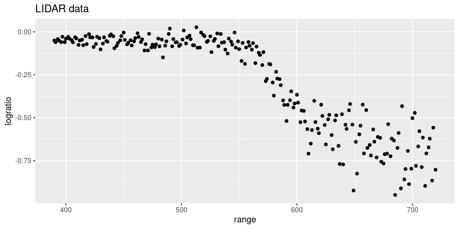
Figure 9.1: LIDAR measurements in the lidar dataset.

A first approach to developing a smooth function to fit the lidar dataset is by using linear combinations of smooth functions on the covariates. The set of functions is called a basis of functions. For example, polynomials up to a certain degree can be easily introduced into the linear predictor by using the I() function in the formula. Alternatively, the poly() function can be used to compute orthogonal polynomials on a covariate up to a certain degree.

Before fitting the model we will create a synthetic dataset with values of range between 390 and 720 (with a step of 5) and NA values, so that these are predicted with INLA (see Section 12.3 for details):

xx <- seq(390, 720, by = 5)
# Add data for prediction
new.data <- cbind(range = xx, logratio = NA)
new.data <- rbind(lidar, new.data)

This new dataset will allow us to obtain estimates of the fitted curve at regular intervals. Next, a model with a 3-degree polynomial on range will be fit:

m.poly <- inla(logratio ~ 1 + range +  I(range^2) + I(range^3),
  data = new.data, control.predictor = list(compute = TRUE))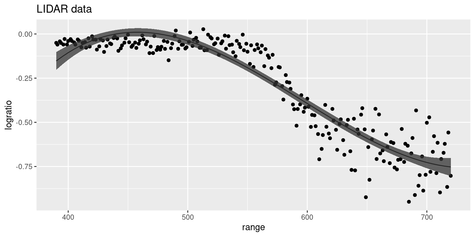

Figure 9.2: Posterior means and 95% credible intervals of the predictive distribution for different values of range using a polynomial of degree 3 fit to the lidar dataset.

The fitted values using these models are shown in Figure 9.2. Although the 3-degree polynomial does a good job of capturing the general variation of the curve, polynomials are not a good choice in general because they produce smooth terms that are fit using all the data because they lack a compact support. Hence, polynomials are too rigid to obtain good local smoothing and the smooth term produced will fit different parts of the dataset with different accuracy. This behavior can be observed in Figure 9.2 at the left edge of the plot where the polynomial does not follow the trend of the data but the polynomial itself.

A better fit could be achieved by using piece-wise functions that vary locally (Ruppert, Wand, and Carroll 2003). A simple approach is to consider broken stick functions. These functions are defined on a number of points or knots so that they have two different slopes that join at the knots. For example, taking knot \(\kappa\), a function can be defined such as

\[ (x - \kappa)_{+} = \left\{ \begin{array}{rl} 0 & x < \kappa\\ x - \kappa & x \geq \kappa \end{array} \right. \]

Note that given a set of knots this definition will produce a particular basis that can be used to model the LIDAR data. Note that \(f(x)\) will be defined by a linear combination of the basis functions and that their coefficients will be estimated as part of the model. This basis is called a linear spline basis.

Hence, given a basis function \(\{(x - \kappa_k)\}_{k=1}^K\) defined by a set of knots \(\{\kappa_k\}_{k=1}^K\), the \(f(\cdot)\) function can be represented as

\[ f(x) = \beta_0 + \beta_ 1 x + \sum_{k=1}^K b_k (x - \kappa_k)_{+} \]

Note that the basis here is made of functions

\[ \{1, x, (x - \kappa_1)_{+}, \ldots, (x- \kappa_K)_{+}\} \]

A truncated power basis of degree \(p\) can be obtained by taking the powers of degree \(p\) of functions \((x - \kappa_k)\), i.e., \((x - \kappa_k)^p_{+}\). This will produce smoother functions with continuous \(p\) derivatives in all the domain but \(\kappa_k\). In this case, function \(f(x)\) is defined as

\[ f(x) = 1 + x + \ldots + x^p + \sum_{k=1}^K b_k (x - \kappa_k)^p_{+} \]

Although this is a first approach to producing local smoothing, broken stick functions may not be smooth enough and other type of functions may be required. For example, instead of piece-wise linear functions, other simple non-linear functions could be used.

In particular, splines (Ruppert, Wand, and Carroll 2003) are a popular option when it comes to producing smooth terms with local smoothing. Splines are smooth functions that are defined using piece-wise functions that join at particular points called knots.

Local smoothing is determined by the number and location of the knots, and they must be chosen with care (Ruppert, Wand, and Carroll 2003). Package splines (R Core Team 2019a) includes several functions for the computation of different types of splines that can be easily combined with INLA to include smooth terms in the model.

For example, function bs() will return a B-spline basis matrix for a polynomial of a given degree. B-splines are preferred to splines because they are computationally more stable. B-splines have the property that they are equivalent to the truncated spline basis of the same degree, i.e., both bases are equivalent and produce the same values in the linear predictor. This means that they will produce the same values of \(f(x)\) but with different coefficients, the B-splines coefficient estimation being more numerically stable (Ruppert, Wand, and Carroll 2003).

In the next example, knots are placed between 400 and 700 at regular intervals using a step of 10. This ensures that the range of values of variable range is covered. The B-spline spline is of degree 3 (i.e., the default).

library("splines")

knots <- seq(400, 700, by = 10)
m.bs3 <- inla(logratio ~ 1 + bs(range, knots = knots),
  data = new.data, control.predictor = list(compute = TRUE))

Note that this model will estimate one coefficient per knot and that, in this case, there are 31 and the model summary is not shown here.

As an alternative to the knots, it is possible to specify the degrees of freedom (Ruppert, Wand, and Carroll 2003) of the spline. Degrees of freedom are related to how flexible a smooth term is in order to capture the the variability in the data.

Natural cubic splines are implemented in function ns(). These types of splines are cubic splines with the added constraint that they are linear at the tail beyond the boundary knots by imposing that the second and third derivatives at the boundary knots (i.e., the ones at the extremes) are equal to zero. In the next example a natural cubic spline with 10 degrees of freedom is used to fit the data (by setting parameter df to 10).

m.ns3 <- inla(logratio ~ 1 + ns(range, df = 10),
  data = new.data, control.predictor = list(compute = TRUE))
summary(m.ns3)

## 
## Call:
##    c("inla(formula = logratio ~ 1 + ns(range, df = 10), data = 
##    new.data, ", " control.predictor = list(compute = TRUE))") 
## Time used:
##     Pre = 0.274, Running = 0.253, Post = 0.0491, Total = 0.577 
## Fixed effects:
##               mean    sd 0.025quant 0.5quant 0.975quant   mode kld
## (Intercept) -0.050 0.032     -0.113   -0.050      0.014 -0.050   0
## 1           -0.010 0.042     -0.093   -0.010      0.073 -0.010   0
## 2           -0.007 0.053     -0.111   -0.007      0.098 -0.007   0
## 3           -0.008 0.048     -0.102   -0.008      0.085 -0.008   0
## 4            0.026 0.051     -0.074    0.026      0.126  0.026   0
## 5           -0.326 0.049     -0.422   -0.326     -0.230 -0.326   0
## 6           -0.554 0.050     -0.652   -0.554     -0.456 -0.554   0
## 7           -0.537 0.049     -0.635   -0.537     -0.440 -0.537   0
## 8           -0.687 0.042     -0.769   -0.687     -0.605 -0.687   0
## 9           -0.656 0.083     -0.819   -0.656     -0.494 -0.656   0
## 10          -0.652 0.038     -0.726   -0.652     -0.578 -0.652   0
## 
## Model hyperparameters:
##                                           mean    sd 0.025quant 0.5quant
## Precision for the Gaussian observations 159.78 15.51     130.83   159.27
##                                         0.975quant   mode
## Precision for the Gaussian observations     191.62 158.25
## 
## Expected number of effective parameters(stdev): 11.21(0.021)
## Number of equivalent replicates : 19.72 
## 
## Marginal log-Likelihood:  173.09 
## Posterior marginals for the linear predictor and
##  the fitted values are computed

In this case we have summarized the output because the number of coefficients is simply 10, in accordance with the degrees of freedom set in function ns() above. Note that there is an extra parameter in the linear predictor which is due to the presence of the intercept.

Figure 9.3 shows both smooth terms estimated using splines. It suggests that it may not be necessary to use as many as 31 when building the spline. The knots used by the second spline are computed using equally spaced quantiles by default:

attr(ns(lidar$range, df = 10), "knots")

## 10% 20% 30% 40% 50% 60% 70% 80% 90% 
## 423 456 489 522 555 588 621 654 687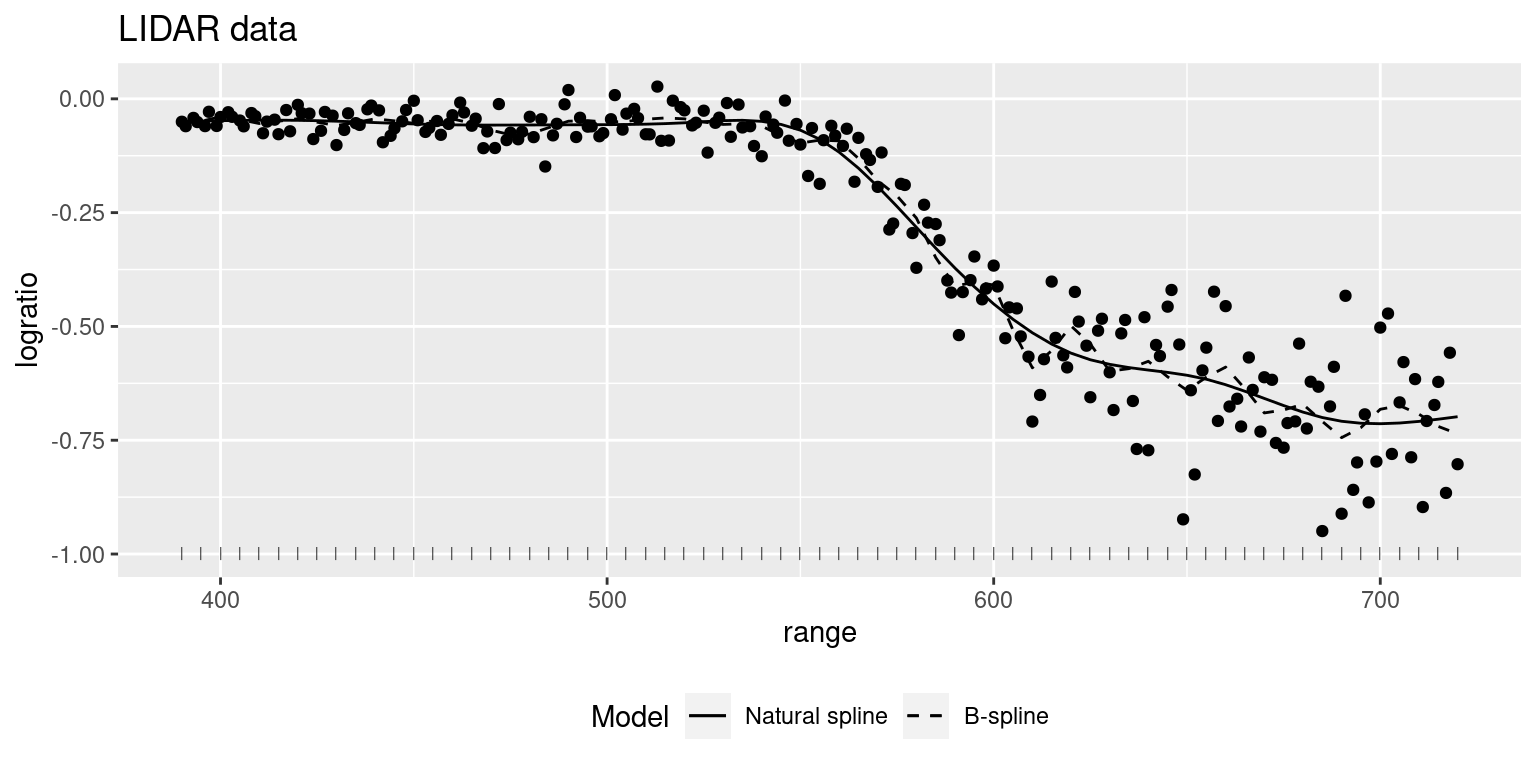

Figure 9.3: Smooth term fit to the lidar using splines of order 3. Knots are displayed at the bottom as tick marks.

Hence, it is clear that using too many knots will make the smooth term overfit the data, while using too few knots will most likely produce biased estimates (Ruppert, Wand, and Carroll 2003).

The need for more or fewer knots can be assessed by looking at the estimates of the coefficients of the spline. Figure 9.4 shows the posterior means and 95% credible intervals on the 3-degree B-spline used above.

It is clear from that plot that most of the terms in the linear predictor can probably be removed without compromising model fitting. In addition, the values of the coefficients seem to follow the shape of the scatterplot of the data, with values close to zero in the regions where the data are more or less constant. Coefficients are away from zero in the regions where data change shape and show more variability.

Hence, it seems necessary to find a way to constrain or penalize the knots and coefficients of the spline so that it is not unnecessarily complex. This can be achieved by resorting to penalized splines or P-splines (Ruppert, Wand, and Carroll 2003; Hastie, Tibshirani, and Friedman 2009), described in the next section.

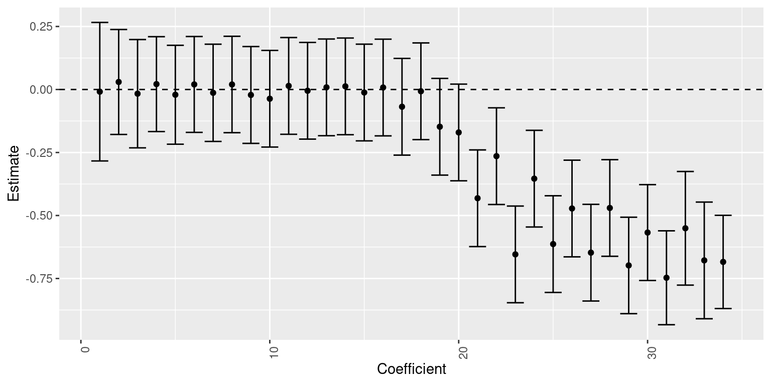
Figure 9.4: Estimates (posterior means and 95% credible intervals) of the coefficients of a 3-degree B-spline.

9.3 Smooth terms with INLA

As seen above, splines provide a good way to include smooth terms in the linear predictor. However, splines have the problem of the selection of the number and position of the knots. Depending on the number and location, splines may overfit the data. As described in Ruppert, Wand, and Carroll (2003), it may be necessary to constrain the influence of the knots by imposing further constraints on the spline coefficients.

Typically, this can be re-formulated as an optimization problem

\[ \min\ \sum_{i=1}^n(y_i - f(x_i))^2 \]

subject to

\[ \sum_{k=1}^p b_k^2 < C \] with \(C\) being a positive constant that controls the degree of shrinkage of the coefficients. Small values of \(C\) will produce small estimates of the coefficients, while very large values will produce estimates that are close to the maximum likelihood estimates (Hastie, Tibshirani, and Friedman 2009; James et al. 2013). Note that only coefficients \(\{b_k\}_{k=1}^K\) are used in the penalty term.

This is equivalent to minimizing the term

\[ \min \sum_{i=1}^n(y_i - f(x_i))^2 + \lambda (\sum_{k=1}^p b_k^2) \] for a fixed parameter \(\lambda >0\). This parameter can be set using cross-validation (Ruppert, Wand, and Carroll 2003; Hastie, Tibshirani, and Friedman 2009; James et al. 2013).

In a Bayesian framework including the penalty term is equivalent to setting a specific prior on the coefficients of the covariates (see, for example, Fahrmeir and Kneib 2011).

For equidistant knots \(\{(\kappa_0, \ldots, \kappa_K)\}\) the prior is on the differences:

\[ f(\kappa_{i + 1}) - f(\kappa_i) \sim N(0, \tau),\ i = 1,\ldots, K-1 \]

which is equivalent to setting a rw1 prior on \(f(\kappa_i)\).

Alternatively, when the prior is on the second order differences

\[ f(\kappa_{i + 1}) - 2 f(\kappa_i) + f(\kappa_{i-1}) \sim N(0, \tau),\ i=2,\ldots,K \]

This is equivalent to setting a rw2 prior on the coefficients.

Hence, latent effects rw1 and rw2 can be used to include smooth terms on the covariates. The elements of the latent effect represent the values of the smooth term.

In the next example, a rw1 latent effect is used. Note that constr is set to FALSE and that, for this reason, the intercept is not included in the linear predictor.

library("INLA")
m.rw1 <- inla(logratio ~ -1 + f(range, model = "rw1", constr = FALSE),
  data = lidar, control.predictor = list(compute = TRUE))
summary(m.rw1)

## 
## Call:
##    c("inla(formula = logratio ~ -1 + f(range, model = \"rw1\", constr 
##    = FALSE), ", " data = lidar, control.predictor = list(compute = 
##    TRUE))" ) 
## Time used:
##     Pre = 0.21, Running = 0.783, Post = 0.0299, Total = 1.02 
## Random effects:
##   Name     Model
##     range RW1 model
## 
## Model hyperparameters:
##                                            mean      sd 0.025quant
## Precision for the Gaussian observations  166.64   17.20     135.01
## Precision for range                     4408.48 1358.58    2287.49
##                                         0.5quant 0.975quant    mode
## Precision for the Gaussian observations   165.90     202.69  164.59
## Precision for range                      4230.93    7572.85 3894.04
## 
## Expected number of effective parameters(stdev): 27.75(4.67)
## Number of equivalent replicates : 7.96 
## 
## Marginal log-Likelihood:  251.74 
## Posterior marginals for the linear predictor and
##  the fitted values are computed

Similarly, a rw2 model can be used to fit a spline to the data:

m.rw2 <- inla(logratio ~ -1 + f(range, model = "rw2", constr = FALSE),
  data = lidar, control.predictor = list(compute = TRUE))
summary(m.rw2)

## 
## Call:
##    c("inla(formula = logratio ~ -1 + f(range, model = \"rw2\", constr 
##    = FALSE), ", " data = lidar, control.predictor = list(compute = 
##    TRUE))" ) 
## Time used:
##     Pre = 0.195, Running = 0.764, Post = 0.0297, Total = 0.988 
## Random effects:
##   Name     Model
##     range RW2 model
## 
## Model hyperparameters:
##                                              mean       sd 0.025quant
## Precision for the Gaussian observations    159.28    15.80     130.07
## Precision for range                     165927.62 51964.52   84509.71
##                                          0.5quant 0.975quant      mode
## Precision for the Gaussian observations    158.65     192.22    157.59
## Precision for range                     159291.21  286249.23 146560.77
## 
## Expected number of effective parameters(stdev): 20.30(1.68)
## Number of equivalent replicates : 10.89 
## 
## Marginal log-Likelihood:  318.99 
## Posterior marginals for the linear predictor and
##  the fitted values are computed

Figure 9.5 shows the lidar dataset together with the fitted values under a rw1 and rw2 latent effects. Predictions seem very similar but, as expected, using a rw2 smooth term provides a smoother function.

Note that this assumes that all the knots are regularly spaced. For the case of irregularly placed data, it is possible to use function inla.group() to bin data into groups according to the values of the covariate. The way in which values are grouped can be set with the method argument, that can be either "cut" (the default) or "quantile". Option "cut" splits the data using equal length intervals, while option "quantile" uses equidistant quantiles in the probability space.

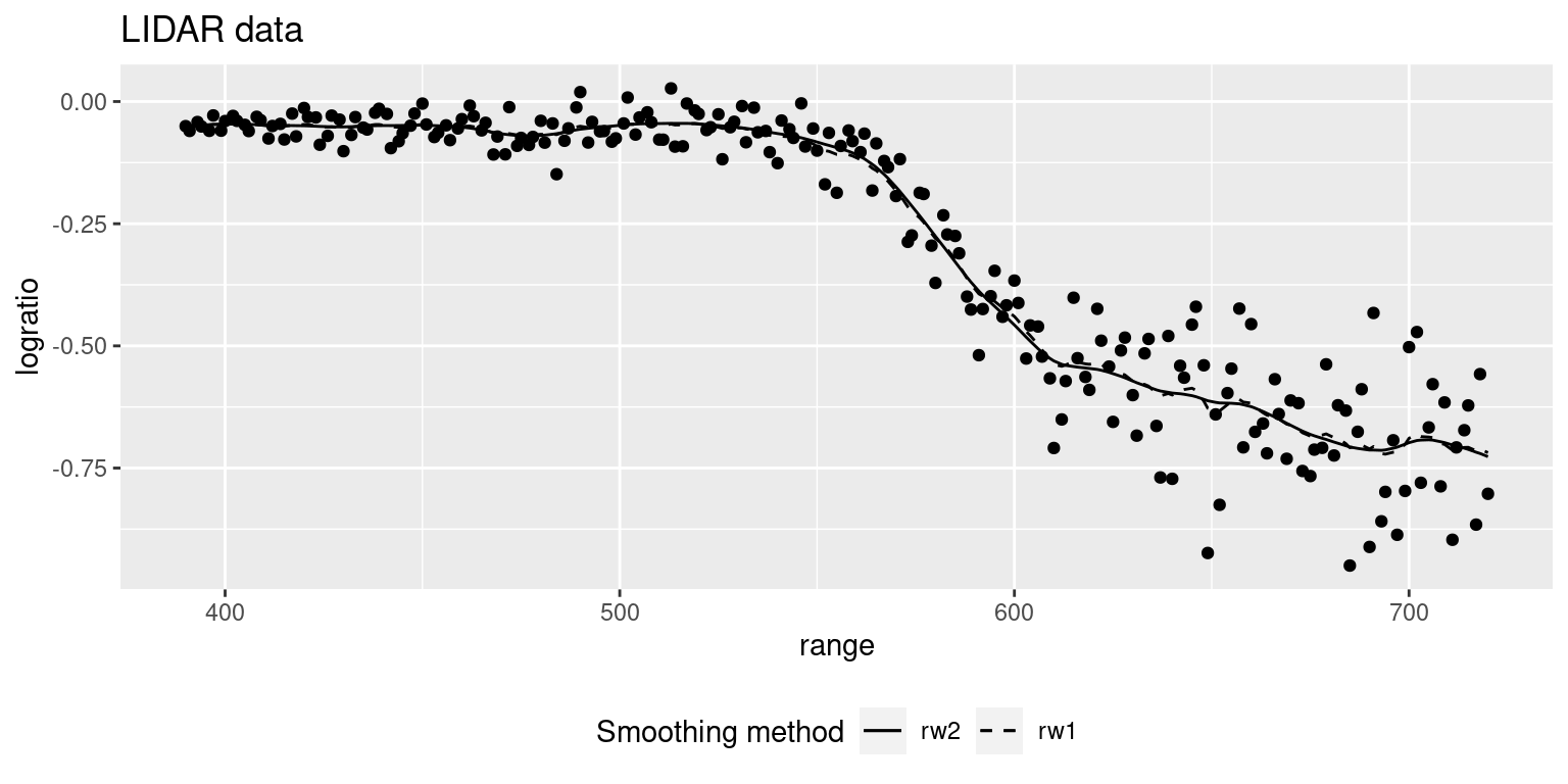
Figure 9.5: LIDAR data together with two smooth estimates (e.g., posterior means) based on rw1 and rw2 effects.

For example, to split the data into 20 groups using equally spaced quantiles the code is:

lidar$range.grp <- inla.group(lidar$range, n = 20, method = "quantile")
summary(lidar$range.grp)

##    Min. 1st Qu.  Median    Mean 3rd Qu.    Max. 
##     394     477     546     555     633     716

The binned data can be see in Figure 9.6. Note that this does not guarantee that the new values of range are equally spaced, but it will help to reduce the number of knots used in the estimation of the smoothing effect.

The newly created variable range.grp can then be used to define the smooth term in the call to inla() inside the f() function. In the next models, this is employed to fit rw1 and rw2 models to the data:

m.grp.rw1 <- inla(logratio ~ -1 + f(range.grp, model = "rw1", constr = FALSE),
  data = lidar, control.predictor = list(compute = TRUE))
summary(m.grp.rw1)

## 
## Call:
##    c("inla(formula = logratio ~ -1 + f(range.grp, model = \"rw1\", 
##    constr = FALSE), ", " data = lidar, control.predictor = 
##    list(compute = TRUE))" ) 
## Time used:
##     Pre = 0.196, Running = 0.418, Post = 0.0269, Total = 0.641 
## Random effects:
##   Name     Model
##     range.grp RW1 model
## 
## Model hyperparameters:
##                                            mean      sd 0.025quant
## Precision for the Gaussian observations  155.87   15.30     127.16
## Precision for range.grp                 4194.49 1403.65    2041.25
##                                         0.5quant 0.975quant    mode
## Precision for the Gaussian observations   155.49     187.13  155.13
## Precision for range.grp                  3999.05    7506.97 3627.23
## 
## Expected number of effective parameters(stdev): 16.30(0.976)
## Number of equivalent replicates : 13.56 
## 
## Marginal log-Likelihood:  238.13 
## Posterior marginals for the linear predictor and
##  the fitted values are computed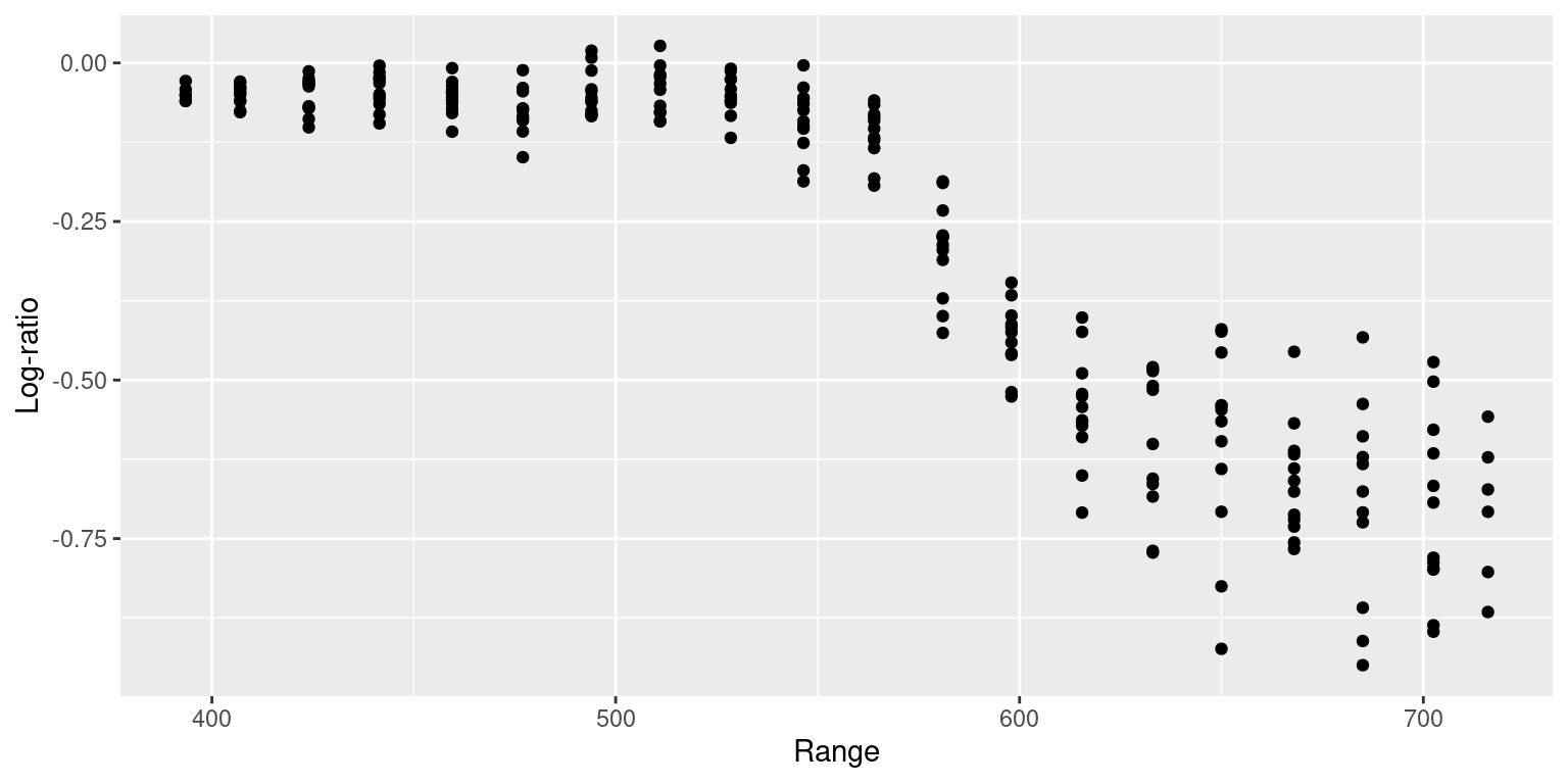

Figure 9.6: Observations of the LIDAR dataset binned according to variable range.

m.grp.rw2 <- inla(logratio ~ -1 + f(range.grp, model = "rw2", constr = FALSE),
  data = lidar, control.predictor = list(compute = TRUE))
summary(m.grp.rw2)

## 
## Call:
##    c("inla(formula = logratio ~ -1 + f(range.grp, model = \"rw2\", 
##    constr = FALSE), ", " data = lidar, control.predictor = 
##    list(compute = TRUE))" ) 
## Time used:
##     Pre = 0.197, Running = 0.496, Post = 0.027, Total = 0.72 
## Random effects:
##   Name     Model
##     range.grp RW2 model
## 
## Model hyperparameters:
##                                              mean       sd 0.025quant
## Precision for the Gaussian observations    154.60    15.25     126.37
## Precision for range.grp                 170344.21 54708.73   83859.33
##                                          0.5quant 0.975quant      mode
## Precision for the Gaussian observations    154.02     186.34    153.05
## Precision for range.grp                 163722.02  296925.58 150611.60
## 
## Expected number of effective parameters(stdev): 18.45(0.498)
## Number of equivalent replicates : 11.98 
## 
## Marginal log-Likelihood:  273.06 
## Posterior marginals for the linear predictor and
##  the fitted values are computed

Figure 9.7 shows the smooth terms estimated with the previous two models. They give very similar fits. The plot has also included the original data (in black) and the binned data (in gray). As compared to the previous models seen in Figure 9.5, the models fit to the binned data seem to be less smooth than the previous ones.

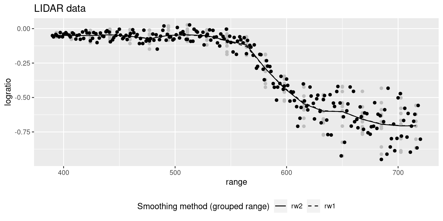
Figure 9.7: Smooth curve fit to the binned dataset on the actual dataset. Original data are shown in black and binned data in gray.

9.4 Smoothing with SPDE

For the case of irregularly spaced data or knots, it is possible to build smooth terms using other latent effects in INLA. In particular, the spde latent effect described in Chapter 7 can also be used in one dimension. In this case, the effect models a Matérn process in one dimension with correlation matrix

\[ Cov(d_{ij}) = \frac{1}{\tau}\frac{2^{1-\nu}}{\Gamma(\nu)}(\kappa d_{ij})^{\nu}K_{\nu}(\kappa d_{ij}) \]

Here, \(d_{ij}\) is the distance between observations \(i\) and \(j\), \(\nu > 0\) a smoothness parameter, \(\kappa >0\) a scale parameter, \(\Gamma(\cdot)\) is the Gamma function and \(K_{\nu}(\cdot)\) is the modified Bessel function of the second kind.

This is described in detail in Krainski et al. (2018), Chapter 2. Usually, the smoothness parameter is fixed and only the precision and the effective range, which is \(\sqrt{8\nu} / \kappa\), are estimated. We describe now how to fit this model, for which we will rely on some of the contents described in Chapter 7 to define the model. Note that the focus now is in modeling in one dimension instead of in spatial models (that are defined in two dimensions). Furthermore, being familiar with Krainski et al. (2018) will be helpful now.

First of all, a set of knots to define the spde model is defined to create a mesh in one dimension and compute the projector matrix:

mesh1d <- inla.mesh.1d(seq(390, 720, by = 20)) 
A1 <- inla.spde.make.A(mesh1d, lidar$range)

Next, the spde model is defined.

spde1 <- inla.spde2.matern(mesh1d, constr = FALSE)
spde1.idx <- inla.spde.make.index("x", n.spde = spde1$n.spde)

In order to fit the model and predict the curve at some points, two data stacks (see Section 7.3) need to be created. The first one includes the data to fit the model:

stack <- inla.stack(data = list(y = lidar$logratio),
  A = list(1, A1),
  effects = list(Intercept = rep(1, nrow(lidar)), spde1.idx),
  tag = "est")

The second stack refers to the points at which the function needs to be estimated. In this case, the points span the values of range with a step of 5 units between each two consecutive values:

# Predict at a finer grid
xx <- seq(390, 720, by = 5)
A.xx <- inla.spde.make.A(mesh1d, xx)
stack.pred <- inla.stack(data = list(y = NA),
  A = list(1, A.xx),
  effects = list(Intercept = rep(1, length(xx)), spde1.idx),
  tag = "pred")

Both data stacks must be put together using function inla.stack().

joint.stack <- inla.stack(stack, stack.pred)

The model is defined now. The formula does not include an intercept because it has been included within the data stack in order to make prediction easier to compute:

formula <- y ~ -1 + f(x, model = spde1)

Then, the inla() function is called to fit the model:

m.spde <- inla(formula, data = inla.stack.data(joint.stack),
  control.predictor = list(A = inla.stack.A(joint.stack), compute = TRUE)
)

Figure 9.8 shows the smooth term fitted to the data using the SPDE model. The fitted curve seems very similar to the ones obtained with rw1and rw2 models. However, 95% credible intervals seem to be narrower. This shows that the hypothesis of constant variance does not hold for this data. Hence, a family that does not assume a constant variance could also be used to model this data.

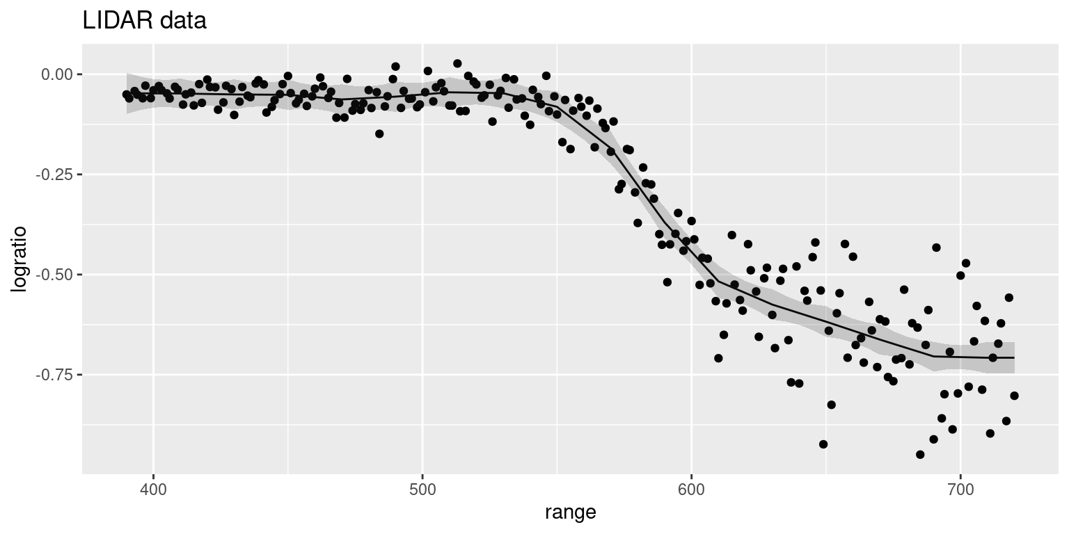
Figure 9.8: Smoothing of LIDAR data using a SPDE in one dimension. The solid line represents the posterior mean and the shaded area is the 95% credible interval of the predictive distribution on range.

9.5 Non-Gaussian models

So far, models for a Gaussian response have been considered. However, the models presented in this chapter can be easily extended to consider the non-Gaussian case. In particular, generalized linear models with smooth terms can be considered. This means that the mean of the non-Gaussian distribution is linked to the linear predictor using an appropriate function. As an example, we will consider an example based on a binomial likelihood using dose-response data.

Dose-response data are a typical example in which the use of a smooth term to explain the relationship between the dose and the number of events is required. Hence, non-parametric methods may be useful to learn the shape of the function that governs this relationship.

The H.virescens dataset (Venables and Ripley 2002) in the drc package (Ritz et al. 2015) contains data from a dose-response experiment in which moths of the tobacco budworm (Heliothis virescens) were exposed for three days to different doses of the pyrethroid trans-cypermethrin (an insecticide). Table 9.2 describes the variables in the dataset.

Table 9.2: Variables in the H.virescens dataset.

Variable	Description
dose	Dose values (in \(\mu\)g).
numdead	Number of dead or knock-down moths.
total	Total number of moths.
sex	Sex (M for male, F for female).

Data can be loaded and summarized as follows:

library("drc")

data(H.virescens)
levels(H.virescens$sex) <- c("Female", "Male")
summary(H.virescens)

##       dose         numdead          total        sex   
##  Min.   : 1.0   Min.   : 0.00   Min.   :20   Female:6  
##  1st Qu.: 2.0   1st Qu.: 3.50   1st Qu.:20   Male  :6  
##  Median : 6.0   Median : 9.50   Median :20             
##  Mean   :10.5   Mean   : 9.25   Mean   :20             
##  3rd Qu.:16.0   3rd Qu.:13.75   3rd Qu.:20             
##  Max.   :32.0   Max.   :20.00   Max.   :20

Dose-response data are typically non-linear because of the effect of the drug administered to the subjects in the study. Furthermore, this data are typically analyzed using a binomial distribution. In the next model, sex is included as control variable and sex is modeled using a rw1 latent effect:

vir.rw1 <- inla(numdead ~ -1 + f(dose, model = "rw1", constr = FALSE) + sex,
  data = H.virescens, family ="binomial", Ntrial = total,
  control.predictor = list(compute = TRUE))
summary(vir.rw1)

## 
## Call:
##    c("inla(formula = numdead ~ -1 + f(dose, model = \"rw1\", constr = 
##    FALSE) + ", " sex, family = \"binomial\", data = H.virescens, 
##    Ntrials = total, ", " control.predictor = list(compute = TRUE))") 
## Time used:
##     Pre = 0.224, Running = 0.0778, Post = 0.0206, Total = 0.322 
## Fixed effects:
##             mean    sd 0.025quant 0.5quant 0.975quant   mode kld
## sexFemale -0.532 22.36     -44.43   -0.532      43.34 -0.532   0
## sexMale    0.532 22.36     -43.37    0.531      44.40  0.532   0
## 
## Random effects:
##   Name     Model
##     dose RW1 model
## 
## Model hyperparameters:
##                    mean   sd 0.025quant 0.5quant 0.975quant mode
## Precision for dose 4.07 3.07      0.645     3.27      12.09 1.96
## 
## Expected number of effective parameters(stdev): 5.75(0.447)
## Number of equivalent replicates : 2.09 
## 
## Marginal log-Likelihood:  -36.49 
## Posterior marginals for the linear predictor and
##  the fitted values are computed

Another model using a rw2 model is fit:

vir.rw2 <- inla(numdead ~ -1 + f(dose, model = "rw2", constr = FALSE) + sex,
  data = H.virescens, family = "binomial", Ntrial = total,
  control.predictor = list(compute = TRUE))
summary(vir.rw2)

## 
## Call:
##    c("inla(formula = numdead ~ -1 + f(dose, model = \"rw2\", constr = 
##    FALSE) + ", " sex, family = \"binomial\", data = H.virescens, 
##    Ntrials = total, ", " control.predictor = list(compute = TRUE))") 
## Time used:
##     Pre = 0.217, Running = 0.0725, Post = 0.0216, Total = 0.311 
## Fixed effects:
##             mean    sd 0.025quant 0.5quant 0.975quant   mode kld
## sexFemale -0.527 22.36     -44.43   -0.528      43.34 -0.527   0
## sexMale    0.527 22.36     -43.38    0.527      44.39  0.527   0
## 
## Random effects:
##   Name     Model
##     dose RW2 model
## 
## Model hyperparameters:
##                       mean      sd 0.025quant 0.5quant 0.975quant  mode
## Precision for dose 3608.70 8982.06      39.97   783.39   28970.09 81.64
## 
## Expected number of effective parameters(stdev): 4.19(0.646)
## Number of equivalent replicates : 2.87 
## 
## Marginal log-Likelihood:  -25.38 
## Posterior marginals for the linear predictor and
##  the fitted values are computed

The models fit to the data are displayed in Figure 9.9. Both models provide very similar estimates of the dose-response effect. Note that the fitted values are shown in Figure 9.10.

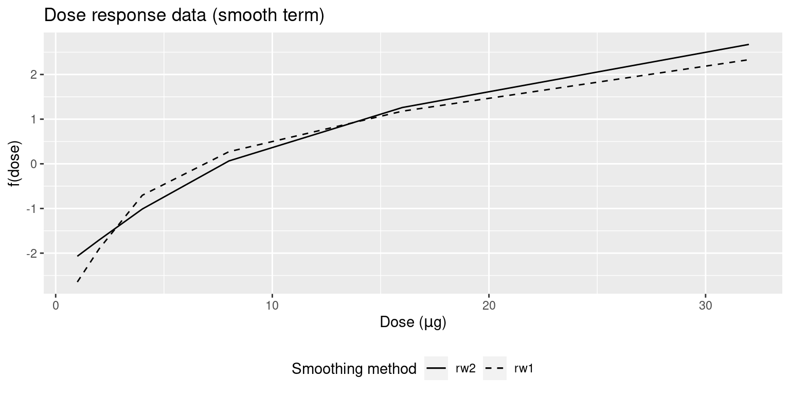
Figure 9.9: Posterior means of the random effects (rw1 or rw2) of the models fit to the dose-response dataset.

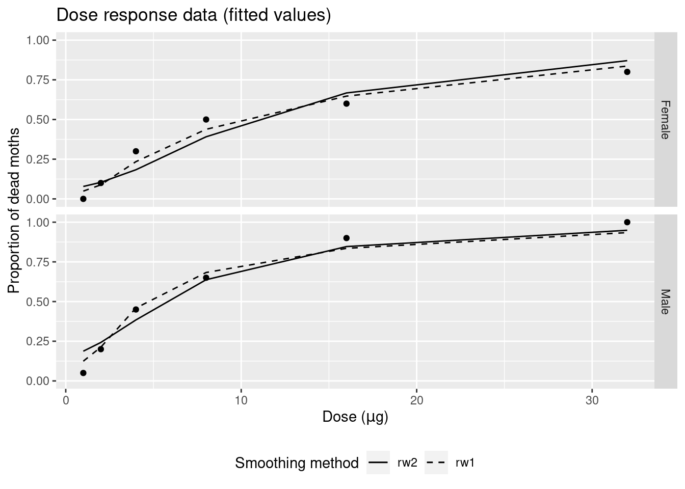
Figure 9.10: Posterior means of the random effects of the models fit to the dose-response dataset.

9.6 Final remarks

This chapter has covered different models for including smooth terms on the covariates in the linear predictor. Smoothing in two dimensions is described in Chapter 7, and some space-time models are also covered in Chapter 8. Wang, Ryan, and Faraway (2018) describe in detail other types of smoothing functions not covered here, such as thin plate splines.

INLA is flexible enough regarding the types of latent effects that can be included. Other types of smooth functions can be implemented using the different frameworks to extend the latent effects implemented in INLA described in Chapter 11.

References

Fahrmeir, Ludwig, and Thomas Kneib. 2011. Bayesian Smoothing Regression for Longitudinal, Spatial and Event History Data. New York: Oxford University Press.

Hastie, Trevor, Robert Tibshirani, and Jerome Friedman. 2009. The Elements of Statistical Learning. 2nd ed. New York: Springer.

Holst, Ulla, Ola Hössjer, Claes Björklund, Pär Ragnarson, and Hans Edner. 1996. “Locally Weighted Least Squares Kernel Regression and Statistical Evaluation of LIDAR Measurements.” Environmetrics 7 (4): 401–16. https://doi.org/10.1002/(SICI)1099-095X(199607)7:4<401::AID-ENV221>3.0.CO;2-D.

James, Gareth, Daniela Witten, Trevor Hastie, and Robert Tibshirani. 2013. An Introduction to Statistical Learning. New York: Springer.

Krainski, Elias T., Virgilio Gómez-Rubio, Haakon Bakka, Amanda Lenzi, Daniela Castro-Camilo, Daniel Simpson, Finn Lindgren, and Håvard Rue. 2018. Advanced Spatial Modeling with Stochastic Partial Differential Equations Using R and INLA. Boca Raton, FL: Chapman & Hall/CRC.

R Core Team. 2019a. R: A Language and Environment for Statistical Computing. Vienna, Austria: R Foundation for Statistical Computing. https://www.R-project.org/.

Ritz, C., F. Baty, J. C. Streibig, and D. Gerhard. 2015. “Dose-Response Analysis Using R.” PLOS ONE 10 (e0146021, 12). http://journals.plos.org/plosone/article?id=10.1371/journal.pone.0146021.

Ruppert, David, M. P. Wand, and R. J. Carroll. 2003. Semiparametric Regression. New York: Cambridge University Press.

Venables, W. N., and B. D. Ripley. 2002. Modern Applied Statistics with S. Fourth. New York: Springer.

Wand, Matt. 2018. SemiPar: Semiparametic Regression. https://CRAN.R-project.org/package=SemiPar.

Wang, Xiaofeng, Yu Yue Ryan, and Julian J. Faraway. 2018. Bayesian Regression Modeling with Inla. Boca Raton, FL: Chapman & Hall/CRC.