Chapter 12 Missing Values and Imputation
12.1 Introduction
Missing observations are common in real life datasets. Values may not be recorded for a number of reasons. For example, environmental data is often not recorded due to failures in measurement devices or instruments. In clinical trials, survival times and other covariates may be missing because of patient’s drop-out.
The literature on missing values is ample. To mention a few, Little and Rubin (2002)
provides a nice overview of missing values and imputation. Buuren (2018)
gives a more recent description of the area, which includes examples using R
code. A curated list of R packages for missing data is available in the
Missing data CRAN Task View available at
https://cran.r-project.org/web/views/MissingData.html.
In general, missing values can seldom be ignored. Models that include a way to account for missing data should be preferred to simply ignoring the missing observations. When missing values can be modeled from the observed data, imputation models can be used to provide estimates of the missing observations. Models can be extended to incorporate a sub-model for the imputation.
The different mechanisms that lead to missing observations in the data are
introduced in Section 12.2. INLA can fit models with missing
observations in the response by computing their predictive distribution, as
discussed in Section 12.3. In principle, INLA cannot directly
handle missing observations in the covariates, as they are part of the latent
field, but imputation of missing covariates using different methods is
discussed in Section 12.4. Multiple imputation of missing
observations in the covariates using INLA within MCMC is described in Section
12.5.
12.2 Missingness mechanism
Dealing with missing observations usually requires prior reflection on how the data went missing and the missingness mechanism. Depending on the reasons why the data has missing observations the statistical analysis needs to be conducted in one way or another. Little and Rubin (2002) describe the different mechanisms for missing data.
Missing completely at random (MCAR) occurs when the missing data are independent from the observed or unobserved data. This means that the missing values can be ignored and the analysis can be conducted as usual. Missing at random (MAR) occurs when the missing data depends on the observed data. In this case, this can be introduced into the model so that missing observations are imputed as part of the model fitting. Finally, Missing not at random (MNAR) occurs when the missingness mechanism depends on both the observed and missing data. This scenario is difficult to tackle since there is no information about the missingness mechanism and the missing data.
Furthermore, a distinction between missing observations in the response variable or the covariates can be done. The missing observations in the response variable can naturally be predicted as the distribution of the response values is determined by the statistical model to be fit. On the other hand, missing values in the covariates are explanatory variables in the model and it is not always clear how they can be estimated. Similarly, missing indices in the definition of the latent random effects are difficult to handle as it is not always obvious how their values can be filled-in. However, different imputation mechanisms can be considered.
INLA does not allow missing values in the definition of the effects in the
latent field, and this is a practical problem for model fitting. In general,
INLA will not include the fixed or random term in the linear predictor of an
observation if the associate covariate has a value of NA. See
Gómez-Rubio, Cameletti, and Blangiardo (2019) and the FAQ at the INLA website
() for details.
12.3 Missing values in the response
First of all, handling missing observations in the response will be considered. Given that the distribution of the response variable is part of the model, it is possible to predict the missing values by computing their predictive distribution. Given a missing response \(y_m\) its predictive distribution is
\[ \pi(y_m \mid \mathbf{y}_{obs}) = \int \pi(y_m, \bm\theta \mid \mathbf{y}_{obs})d\bm\theta = \int\pi(y_m \mid \mathbf{y}_{obs}, \bm\theta) \pi(\bm\theta \mid \mathbf{y}_{obs})d\bm\theta . \]
INLA will automatically compute the predictive distributions for all
missing values in the response, which should be assigned a NA value when
defining the data.
To illustrate the computation of the predictive distribution of the missing
values in the response the fdgs dataset (in package mice, van Buuren and Groothuis-Oudshoorn 2011) will
be used. This dataset records information of 10030 children measured within
the Fifth Dutch Growth Study 2009 (Schonbeck et al. 2011, 2013).
Table 12.1 shows the different variables in the dataset.
| Variable | Description | # missing |
|---|---|---|
id |
Child unique id number. | 0 |
reg |
Region (a factor with 5 levels). | 0 |
age |
Age (in year). | 0 |
sex |
Sex (boy or girl). |
0 |
hgt |
Height (in cm). | 23 |
wgt |
Weight (in kg). | 20 |
hgt.z |
Re-scaled height (as a Z-score). | 23 |
wgt.z |
Re-scaled weight (as a Z-score). | 20 |
Data can be loaded and summarized as follows:
library("mice")
data(fdgs)
summary(fdgs)
## id reg age sex
## Min. :100001 North: 732 Min. : 0.008 boy :4829
## 1st Qu.:106352 East :2528 1st Qu.: 1.619 girl:5201
## Median :203855 South:2931 Median : 8.085
## Mean :180091 West :2578 Mean : 8.158
## 3rd Qu.:210591 City :1261 3rd Qu.:13.548
## Max. :401955 Max. :21.993
##
## hgt wgt hgt.z wgt.z
## Min. : 46.0 Min. : 2.58 Min. :-4.470 Min. :-5.040
## 1st Qu.: 83.8 1st Qu.: 11.60 1st Qu.:-0.678 1st Qu.:-0.625
## Median :131.5 Median : 27.50 Median :-0.019 Median : 0.026
## Mean :123.9 Mean : 32.38 Mean :-0.006 Mean : 0.046
## 3rd Qu.:162.3 3rd Qu.: 51.10 3rd Qu.: 0.677 3rd Qu.: 0.707
## Max. :208.0 Max. :135.30 Max. : 3.900 Max. : 4.741
## NA's :23 NA's :20 NA's :23 NA's :20Note that several variables in the dataset have missing observations.
In particular, height (hgt) and weight (wgt), which are common variables
used as response or predictors in models.
In order to provide a smaller dataset to speed up computations, only the children with missing values (in height and weight) and another 1000 ones taken at random will be used in the analysis:
# Subset for speed-up and testing
# Subsect 1, observations with NA's
subset1 <- which(is.na(fdgs$wgt) | is.na(fdgs$hgt))

#Subset 2, random sample of 500 individuals
set.seed(1)
subset2 <- sample((1:nrow(fdgs))[-subset1], 1000)
# Subset 1 + subset 2
fdgs.sub <- fdgs[c(subset1, subset2), ]
summary(fdgs.sub)
## id reg age sex hgt
## Min. :100098 North: 78 Min. : 0.071 boy :493 Min. : 46.0
## 1st Qu.:106293 East :275 1st Qu.: 1.743 girl:550 1st Qu.: 86.3
## Median :204306 South:298 Median : 8.594 Median :136.1
## Mean :183214 West :250 Mean : 8.565 Mean :127.0
## 3rd Qu.:211388 City :142 3rd Qu.:14.164 3rd Qu.:165.1
## Max. :401949 Max. :21.884 Max. :199.0
## NA's :23
## wgt hgt.z wgt.z
## Min. : 2.58 Min. :-4.263 Min. :-4.075
## 1st Qu.: 11.96 1st Qu.:-0.668 1st Qu.:-0.652
## Median : 29.00 Median :-0.046 Median :-0.007
## Mean : 33.61 Mean :-0.023 Mean : 0.020
## 3rd Qu.: 53.10 3rd Qu.: 0.645 3rd Qu.: 0.696
## Max. :117.30 Max. : 3.200 Max. : 3.630
## NA's :20 NA's :23 NA's :20Next, a model to predict height based on age and sex is fit to the subset data
set fdgs.sub with INLA. This model includes the options to compute the
predictive distributions of the missing observations in the response by setting
compute = TRUE in argument control.predictor.
library("INLA")
hgt.inla <- inla(hgt ~ age + sex, data = fdgs.sub,
control.predictor = list(compute = TRUE))
summary(hgt.inla)
##
## Call:
## "inla(formula = hgt ~ age + sex, data = fdgs.sub,
## control.predictor = list(compute = TRUE))"
## Time used:
## Pre = 0.394, Running = 0.336, Post = 0.128, Total = 0.858
## Fixed effects:
## mean sd 0.025quant 0.5quant 0.975quant mode kld
## (Intercept) 77.148 0.720 75.735 77.148 78.560 77.148 0
## age 6.023 0.055 5.914 6.023 6.131 6.023 0
## sexgirl -4.716 0.730 -6.149 -4.716 -3.284 -4.716 0
##
## Model hyperparameters:
## mean sd 0.025quant 0.5quant
## Precision for the Gaussian observations 0.007 0.00 0.007 0.007
## 0.975quant mode
## Precision for the Gaussian observations 0.008 0.007
##
## Expected number of effective parameters(stdev): 3.00(0.00)
## Number of equivalent replicates : 340.06
##
## Marginal log-Likelihood: -3976.26
## Posterior marginals for the linear predictor and
## the fitted values are computedIn order to show the predictive distribution, we will obtain first the indices of the first two children with missing values of height in the reduced dataset and show the row names in the original dataset.
hgt.na <- which(is.na(fdgs.sub$hgt))[1:2]
rownames(fdgs.sub)[hgt.na]
## [1] "273" "2034"Next, the summary statistics of the fitted values can be shown
using index hgt.na:
hgt.inla$summary.fitted.values[hgt.na, c("mean", "sd")]## mean sd
## fitted.Predictor.0001 122.25 0.5353
## fitted.Predictor.0005 83.25 0.6830Similarly, a model can be fit to explain weight based on age and sex and to compute the predictive distribution of the missing observations:
wgt.inla <- inla(wgt ~ age + sex, data = fdgs.sub,
control.predictor = list(compute = TRUE),
control.compute = list(config = TRUE))
summary(wgt.inla)
##
## Call:
## c("inla(formula = wgt ~ age + sex, data = fdgs.sub,
## control.compute = list(config = TRUE), ", " control.predictor =
## list(compute = TRUE))")
## Time used:
## Pre = 0.356, Running = 0.315, Post = 0.0693, Total = 0.74
## Fixed effects:
## mean sd 0.025quant 0.5quant 0.975quant mode kld
## (Intercept) 6.259 0.436 5.403 6.259 7.115 6.259 0
## age 3.331 0.034 3.265 3.331 3.397 3.331 0
## sexgirl -2.379 0.446 -3.255 -2.379 -1.503 -2.379 0
##
## Model hyperparameters:
## mean sd 0.025quant 0.5quant
## Precision for the Gaussian observations 0.02 0.001 0.018 0.02
## 0.975quant mode
## Precision for the Gaussian observations 0.021 0.02
##
## Expected number of effective parameters(stdev): 3.00(0.00)
## Number of equivalent replicates : 341.01
##
## Marginal log-Likelihood: -3486.82
## Posterior marginals for the linear predictor and
## the fitted values are computedThis model could be used as a simple imputation mechanism for the missing
values of weight, so that the complete dataset could be used to fit, for
example, another model to explain height based on age, sex, and weight.
Here, we check the posterior means of the predictive distribution of
weight for the first two children with missing values of the variable
wgt:
wgt.na <- which(is.na(fdgs.sub$wgt))
wgt.inla$summary.fitted.values[wgt.na[1:2], c("mean", "sd")]
## mean sd
## fitted.Predictor.0002 23.07 0.3204
## fitted.Predictor.0003 27.62 0.333212.3.1 Joint model with height and weight
The two previous models consider height and weight separately, but it is clear that there is a high correlation between height and weight, which is caused by the age and sex of the child. For this reason, a joint model for height and weight could be proposed to exploit a correlated effect between the coefficients of age in both models.
This can be easily implemented with INLA by using a model with two Gaussian
likelihoods (for height and weight, respectively) and the latent effect
iid2d to include two correlated coefficients in the two parts of the model.
Hence, the model will be the following:
\[ hgt_i = \alpha_h + \beta_h age_i + \beta_{h,1} sex_i + \epsilon_{h,i} \]
\[ wgt_i = \alpha_w + \beta_w age_i + \beta_{w,1} sex_i + \epsilon_{w,i} \]
Here, \(\alpha_h\) and \(\alpha_w\) are model intercepts, \(\beta_h\) and \(\beta_w\)
coefficients on age (which will be correlated), \(\beta_{h,1}\) and
\(\beta_{w,1}\) coefficients on sex, and \(\epsilon_{h,i}\) and \(\epsilon_{w,i}\)
two error terms.
Vector \((\beta_h, \beta_w)^{\top}\) is modeled using a multivariate Gaussian distribution with mean \(c(0, 0)^{\top}\) and covariance matrix
\[ \left[ \begin{array}{cc} 1 / \tau_h & \rho / \sqrt(\tau_h \tau_w)\\ \rho / \sqrt(\tau_h \tau_w) & 1 / \tau_w\\ \end{array} \right] \]
Here, \(\tau_h\) and \(\tau_w\) are the precisions of the coefficients and \(\rho\) is
the correlation parameter, which is between 0 and 1. This model is implemented
in INLA as the iid2d latent effect (see Section 3.3 for
more details). Note that the covariate age will be introduced as a weight of
this latent effect (see below for details) when it is defined with function
f().
First of all, the bivariate response variable needs to be put in a two-column matrix given that the model will be made of two likelihoods (see Section 6.4 for details).
n <- nrow(fdgs.sub)
y <- matrix(NA, nrow = 2 * n, ncol = 2)
y[1:n, 1] <- fdgs.sub$hgt
y[n + 1:n, 2] <- fdgs.sub$wgt
Similarly, given that the model will include two intercepts, these need to be defined explicitly as covariates with all values equal to one. The structure must also be a two-column matrix to have two different intercepts, one for each likelihood.
I <- matrix(NA, nrow = 2 * n, ncol = 2)
I[1:n, 1] <- 1
I[n + 1:n, 2] <- 1
Variable sex needs to be put in a similar format so that the model includes
two separate coefficients in each of the two parts of the model.
SEX <- matrix(NA, nrow = 2 * n, ncol = 2)
SEX[1:n, 1] <- fdgs.sub$sex
SEX[n + 1:n, 2] <- fdgs.sub$sex
Variable age also needs to be put in a different format, but given that
it will be a weight in the iid2d latent effect, it must be passed as a vector
of replicated values:
age.joint <- rep(fdgs.sub$age, 2)Finally, an index vector to indicate which coefficient to use from the iid2d
model is required. This index will be 1 for the first half of observations
(to indicate that the coefficient is \(\beta_h\)) and 2 for the second half (to
indicate that the coefficient is \(\beta_w\)).
idx.age = rep(1:2, each = n)The model is fit and summarized as seen below. Note how the estimates of the
intercepts and the coefficients for sex are very similar to those from the
univariate models.
# Model formula
joint.f <- y ~ -1 + I + f(idx.age, age, model = "iid2d", n = 2) + SEX
# Model fit
fdgs.joint <- inla(joint.f,
  data = list(y = y, I = I, SEX = SEX, age = age.joint, idx.age = idx.age),
  family = rep("gaussian", 2),
  control.predictor = list(compute = TRUE))
# Summary
summary(fdgs.joint)
##
## Call:
## c("inla(formula = joint.f, family = rep(\"gaussian\", 2), data =
## list(y = y, ", " I = I, SEX = SEX, age = age.joint, idx.age =
## idx.age), control.predictor = list(compute = TRUE))" )
## Time used:
## Pre = 0.276, Running = 2.17, Post = 0.101, Total = 2.55
## Fixed effects:
## mean sd 0.025quant 0.5quant 0.975quant mode kld
## I1 81.740 1.272 79.242 81.740 84.236 81.740 0
## I2 8.658 0.773 7.140 8.658 10.174 8.658 0
## SEX1 -4.649 0.729 -6.081 -4.649 -3.219 -4.649 0
## SEX2 -2.377 0.445 -3.250 -2.377 -1.504 -2.377 0
##
## Random effects:
## Name Model
## idx.age IID2D model
##
## Model hyperparameters:
## mean sd 0.025quant 0.5quant
## Precision for the Gaussian observations 0.007 0.000 0.007 0.007
## Precision for the Gaussian observations[2] 0.020 0.001 0.018 0.020
## Precision for idx.age (component 1) 0.309 0.088 0.164 0.301
## Precision for idx.age (component 2) 1.177 0.314 0.640 1.154
## Rho1:2 for idx.age 0.782 0.082 0.601 0.790
## 0.975quant mode
## Precision for the Gaussian observations 0.008 0.007
## Precision for the Gaussian observations[2] 0.021 0.020
## Precision for idx.age (component 1) 0.508 0.284
## Precision for idx.age (component 2) 1.867 1.110
## Rho1:2 for idx.age 0.916 0.810
##
## Expected number of effective parameters(stdev): 5.99(0.003)
## Number of equivalent replicates : 341.13
##
## Marginal log-Likelihood: -7481.61
## Posterior marginals for the linear predictor and
## the fitted values are computedThe coefficients for age are part of the random effects of the model. The
estimates are very similar to the ones obtained in the univariate models. Note
how the standard deviations seem to be slightly smaller.
fdgs.joint$summary.random$idx.age## ID mean sd 0.025quant 0.5quant 0.975quant mode kld
## 1 1 6.024 0.05538 5.915 6.024 6.133 6.024 3.453e-07
## 2 2 3.328 0.03355 3.262 3.328 3.394 3.328 1.345e-07The estimates of height of the children that had missing values are these now:
fdgs.joint$summary.fitted.values[hgt.na, c("mean", "sd")]## mean sd
## fitted.Predictor.0001 122.20 0.5348
## fitted.Predictor.0005 83.19 0.6825In a similar way, the estimates of weight of the children with missing values explored above can also be checked:
fdgs.joint$summary.fitted.values[n + wgt.na[1:2], c("mean", "sd")]## mean sd
## fitted.Predictor.1045 23.08 0.3192
## fitted.Predictor.1046 27.62 0.331912.4 Imputation of missing covariates
As seen in the previous section, the missing values in the response can be handled by computing their predictive distribution and this is possible because the data generating process is specified in the model likelihood. Missing values in the covariates pose a different problem as covariates are supposed to be explanatory variables and the model does not provide any information about the generating process of the covariates. However, imputation models can be proposed by exploiting the correlation among the different observed variables.
A simple approach to tackle missing observations in the covariates is to build a regression model to explain the covariate with the missing observations and plug-in the obtained estimates (e.g., posterior means) from their predictive distributions (Little and Rubin 2002). This approach is simple and easy to implement in most cases, but it ignores the uncertainty about the imputed values.
A better approach would be to include a sub-model for the imputation of missing values within the main model to be fit. This will propagate the uncertainty from the imputed values throughout the model. However, this means than an extra level is required in the model and INLA is not designed to include this (see, for example, Gómez-Rubio, Cameletti, and Blangiardo 2019).
In order to develop an example of the approaches mentioned above to fit models with missing observations in the covariates, we will build a model to explain height based on age, sex and weight. Note that now the missing observations in height are part of the response (and their predictive distributions can be computed) but the missing observations in weight are part of the latent effect.
First of all, a model is fit to the reduced dataset fdgs.sub. Note that this
data.frame contains missing observations of variable wgt, which is in the
linear predictor. Hence, INLA will not remove the rows with the missing
observations in wgt before fitting the model, which means that some
observations are actually not used to estimate the coefficient of wgt. This
model will provide a baseline to compare to other approaches.
hgt.noimp <- inla(hgt ~ 1 +  age + sex + wgt, data = fdgs.sub)
summary(hgt.noimp)
##
## Call:
## "inla(formula = hgt ~ 1 + age + sex + wgt, data = fdgs.sub)"
## Time used:
## Pre = 0.193, Running = 0.221, Post = 0.0198, Total = 0.434
## Fixed effects:
## mean sd 0.025quant 0.5quant 0.975quant mode kld
## (Intercept) 75.308 0.740 73.855 75.308 76.760 75.308 0
## age 4.971 0.147 4.681 4.971 5.260 4.971 0
## sexgirl -4.012 0.716 -5.417 -4.012 -2.608 -4.012 0
## wgt 0.318 0.041 0.236 0.318 0.399 0.318 0
##
## Model hyperparameters:
## mean sd 0.025quant 0.5quant
## Precision for the Gaussian observations 0.008 0.00 0.007 0.008
## 0.975quant mode
## Precision for the Gaussian observations 0.009 0.008
##
## Expected number of effective parameters(stdev): 4.00(0.00)
## Number of equivalent replicates : 255.03
##
## Marginal log-Likelihood: -3954.24Next, we take the previous model fit to wgt to plug-in the posterior
means of the missing observations into a new imputed data set called
fdgs.imp:
fdgs.plg <- fdgs.sub
fdgs.plg$wgt[wgt.na] <- wgt.inla$summary.fitted.values[wgt.na, "mean"]
Note how the values of wgt in the new dataset fdgs.plg do not contain any NA’s:
summary(fdgs.plg$wgt)## Min. 1st Qu. Median Mean 3rd Qu. Max.
## 2.58 12.00 29.00 33.54 52.90 117.30This new dataset is used to fit a new model where there are only missing observations in the response:
hgt.plg <- inla(hgt ~ 1 +  age + sex + wgt, data = fdgs.plg,
control.predictor = list(compute = TRUE))
summary(hgt.plg)
##
## Call:
## "inla(formula = hgt ~ 1 + age + sex + wgt, data = fdgs.plg,
## control.predictor = list(compute = TRUE))"
## Time used:
## Pre = 0.215, Running = 0.384, Post = 0.0747, Total = 0.674
## Fixed effects:
## mean sd 0.025quant 0.5quant 0.975quant mode kld
## (Intercept) 73.982 0.751 72.507 73.982 75.455 73.982 0
## age 4.348 0.171 4.012 4.348 4.683 4.348 0
## sexgirl -3.490 0.705 -4.874 -3.490 -2.107 -3.490 0
## wgt 0.503 0.049 0.407 0.503 0.599 0.503 0
##
## Model hyperparameters:
## mean sd 0.025quant 0.5quant
## Precision for the Gaussian observations 0.008 0.00 0.007 0.008
## 0.975quant mode
## Precision for the Gaussian observations 0.009 0.008
##
## Expected number of effective parameters(stdev): 4.00(0.00)
## Number of equivalent replicates : 255.03
##
## Marginal log-Likelihood: -3932.10
## Posterior marginals for the linear predictor and
## the fitted values are computedThe estimates of height for the two first children with missing observations is:
hgt.plg$summary.fitted.values[hgt.na[1:2], ]## mean sd 0.025quant 0.5quant 0.975quant mode
## fitted.Predictor.0001 118.20 0.6431 116.94 118.20 119.46 118.20
## fitted.Predictor.0005 82.63 0.6530 81.35 82.63 83.91 82.63Note how the estimates of the model effects have changed. It is worth mentioning that the last model has included the subjects that had missing observations of the weight to estimate its coefficient because they have now been imputed.
Including the full imputation mechanism in the model will require a sub-model
within the main model. This is not currently implemented in INLA but this can
be easily implemented as a new latent effect with the methods described in
Section 11 (Gómez-Rubio, Cameletti, and Blangiardo 2019). Alternatively,
Cameletti, Gómez-Rubio, and Blangiardo (2019) propose sampling from the predictive distribution of the
imputation model, fitting models conditional on this imputed values and then
using Bayesian model average on all the models fit to estimate a final model.
The resulting model will account for the uncertainty of the imputation
mechanism. In the next sections we provide different solutions to this problem
by using a sample from the imputation model and by implementing an imputation
mechanism using INLA within MCMC (Gómez-Rubio and HRue 2018).
12.4.1 Sampling from the imputation model
When imputed values are plugged-into the data the actual model fit is conditional on these values and therefore, ignores the uncertainty about the imputation process. The marginals resulting from this model can be represented as
\[ \pi(\theta_t \mid \mathbf{y}_{obs}, \mathbf{x}_{mis} = x^*_{mis}) \] where \(x^*_{mis}\) are the plugged-in values of the missing covariates and \(\theta_t\) represents a latent effect or hyperparameter in the model.
Note that the imputation model will produce predictive distributions \(\pi_I(\mathbf{x}_{mis} \mid \mathbf{y}_{imp})\), where \(\mathbf{y}_{imp}\) are the observed data used in the imputation model. This model may have further parameters \(\bm\theta_{I}\), for which posterior marginals can be obtained (but these are not really of interest now).
The posterior distribution of the parameters in the model can be obtained by integrating out the missing observations with regard to the imputation model, i.e.,
\[ \pi(\theta_t \mid \mathbf{y}_{obs}) = \int\pi(\theta_t, \mathbf{x}_{mis} \mid \mathbf{y}_{obs}) d\mathbf{x}_{mis} = \int\pi(\theta_t \mid \mathbf{x}_{mis}, \mathbf{y}_{obs}) \pi(\mathbf{x}_{mis} \mid \mathbf{y}_{obs}) d\mathbf{x}_{mis} \]
Note that now \(\mathbf{y}_{obs}\) refers to the observed data for the main model and the imputation model, i.e., \(\mathbf{y}_{obs} = (\mathbf{y}, \mathbf{y}_{imp})\). \(\mathbf{y}\) now includes the response variables plus any other fully observed covariates in the main model. The previous equation makes it clear that the predictive distribution of the missing observations is informed by the observed data in the general model and the data used in the imputation model.
As \(\pi(\mathbf{x}_{mis} \mid \mathbf{y}_{obs})\) is seldom available, it can be replaced by the predictive distribution of \(\mathbf{x}_{mis}\) obtained with the imputation model, i.e., \(\pi_I(\mathbf{x}_{mis} \mid \mathbf{y}_{imp})\). This assumes that \(\mathbf{x}_{mis}\) is only informed by the observed data in the imputation model (\(\mathbf{y}_{imp}\)) and ignores any dependence on the response variable and the main model. Then, the approximation is
\[ \pi(\theta_t \mid \mathbf{y}_{obs}) \simeq \int\pi(\theta_t \mid \mathbf{x}_{mis}, \mathbf{y}_{obs}) \pi_I(\mathbf{x}_{mis} \mid \mathbf{y}_{imp}) d\mathbf{x}_{mis} \]
Hence, the the posterior marginal of \(\theta_t\) can be approximated by sampling \(n_{imp}\) values of \(\mathbf{x}_{mis}\) from their predictive distribution \(\{\mathbf{x}^{(i)}_{mis}\}_{i=1}^{n_m}\) (see discussion in Cameletti, Gómez-Rubio, and Blangiardo 2019):
\[ \pi(\theta_t \mid \mathbf{y}_{obs}) \simeq \frac{1}{n_i} \sum_{i=1}^{n_{imp}}\pi(\theta_t \mid \mathbf{y}_{obs}, \mathbf{x}_{mis} = \mathbf{x}^{(i)}_{mis}) \]
Note that \(\pi(\theta_t \mid \mathbf{y}_{obs}, \mathbf{x}_{mis} = \mathbf{x}^{(i)}_{mis})\) is obtained by fitting a model with INLA in which the missing observations have been set to \(\mathbf{x}^{(i)}_{mis}\).
The following code obtains 50 samples from the posterior distribution
of the imputation model obtained using function inla.posterior.sample()
(see Section 2.7):
n.imp <- 50
wgt.pred <- inla.posterior.sample(n.imp, wgt.inla)
The samples include the linear predictor. For the first set of samples, the values of the imputed weights (i.e., the linear predictor) are:
wgt.pred[[1]]$latent[wgt.na,]## Predictor:2 Predictor:3 Predictor:4 Predictor:6 Predictor:9
## 22.477 27.522 52.876 13.306 7.518
## Predictor:11 Predictor:14 Predictor:15 Predictor:21 Predictor:22
## 11.746 12.493 6.210 17.201 70.037
## Predictor:28 Predictor:29 Predictor:34 Predictor:35 Predictor:36
## 44.484 12.355 23.686 26.014 55.913
## Predictor:37 Predictor:38 Predictor:39 Predictor:40 Predictor:42
## 34.227 37.247 33.164 36.284 37.637The original dataset can be completed with each of the 50 sets of imputed
values and the the model can be fit with INLA:
imp.models <- lapply(1:n.imp, function(i) {
  fdgs.plg$wgt[wgt.na] <- wgt.pred[[i]]$latent[wgt.na, ]
  inla(hgt ~ 1 +  age + sex + wgt, data = fdgs.plg,
    control.predictor = list(compute = TRUE))
})
The fit models can be put together by computing the average model using
Bayesian model averaging (Hoeting et al. 1999). For this, function inla.merge()
is used with equal weights (\(1/n_{imp}\)):
model.imp <- inla.merge(imp.models, rep(1 / n.imp, n.imp))The marginals for the fixed effects and hyperparameters are then extracted to be used later:
marg.fixed <- model.imp$marginals.fixed
marg.hyperpar <- model.imp$marginals.hyperpar
Summary statistics of the marginals of the fixed effects can be obtained as usual:
summary(model.imp)##
## Call:
## "inla(formula = hgt ~ 1 + age + sex + wgt, data = fdgs.plg,
## control.predictor = list(compute = TRUE))"
## Time used:
## Pre = 80.8, Running = 11.2, Post = 5.92, Total = 97.8
## Fixed effects:
## mean sd
## (Intercept) 75.712 2.702
## age 3.722 0.641
## sexgirl -1.869 2.343
## wgt 0.654 0.185
##
## Model hyperparameters:
## mean sd
## Precision for the Gaussian observations 0.013 0.002
##
## Marginal log-Likelihood: -278.21
## Posterior marginals for the linear predictor and
## the fitted values are computedSimilarly, summary statistics of the predictive distribution for the first two children with missing values of height can be obtained using the estimates of the linear predictor:
model.imp$summary.linear.predictor[hgt.na[1:2], ]## mean sd
## Predictor.01 118.7 2.412
## Predictor.05 85.0 2.193Note that if the likelihood is not Gaussian in order to get the estimates of the fitted values the linear predictor needs to be conveniently transformed.
In order to assess the impact of the imputed values of weight in the model, the averaged predictive distribution for a given child with a missing value of height can be compared to the predictive distribution obtained from fitting the models to the 50 imputed values. Figure 12.1 shows the averaged predictive distribution (in black) as well as the different 50 predictive distributions. In this particular case, all of them are very similar.
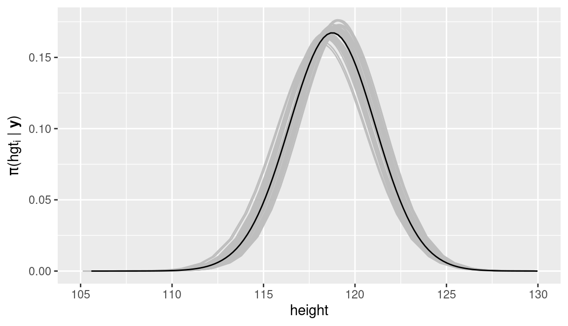
Figure 12.1: Predictive distribution of a missing observation of height in the fdgs dataset in the final average model (black) and predictive distributions from the 50 different models fit to the imputed datasets (gray).
12.5 Multiple imputation of missing values
Gómez-Rubio and HRue (2018) discuss the use of INLA within MCMC to fit models with missing observations. In a Bayesian framework, missing observations can be treated as any other parameter in the model, which means that they need to be assigned a prior distribution (if an imputation model is not provided).
This example will be illustrated using the nhanes2 (Schafer 1997), available
in the mice package (van Buuren and Groothuis-Oudshoorn 2011). The R code reproduced here is taken from
the example in Gómez-Rubio and HRue (2018) and it is available from GitHub (see
Preface for details).
The nhanes2 dataset is a subset of 25 observations from the National Health
and Nutrition Examination Survey (NHANES). Table 12.2 shows the
different variables in this dataset, which can be loaded and summarized as:
library("mice")

data(nhanes2)
summary(nhanes2)
## age bmi hyp chl
## 20-39:12 Min. :20.4 no :13 Min. :113
## 40-59: 7 1st Qu.:22.6 yes : 4 1st Qu.:185
## 60-99: 6 Median :26.8 NA's: 8 Median :187
## Mean :26.6 Mean :191
## 3rd Qu.:28.9 3rd Qu.:212
## Max. :35.3 Max. :284
## NA's :9 NA's :10| Variable | Description |
|---|---|
age |
Age group (numeric, with 1=20-39, 2=40-59 and 3=60+). |
bmi |
Body mass index (in kg / m\(^2\)). |
hyp |
Hypertensive (numeric, with 1=no and 2=yes). |
chl |
Cholesterol level (mg/dL). |
Note how there are missing observations of the body mass index and the cholesterol level. The interest now is to build a model to explain the cholesterol level based on the other variables in the dataset:
\[ chl_i = \alpha + \beta_1 bmi_i + \beta_2 age^{40-59}_i + \beta_3 age^{60+}_i + \epsilon_i,\ i=1, \ldots, 25 \]
Here, \(age^{40-59}_i\) and \(age^{60+}_i\) are indicator variables derived from
age to indicate whether a patient is in age group 40-59 or 60+, respectively.
In addition, \(\alpha\) is the model intercept, \(\beta_j,\ j=1,\ldots, 3\) are
coefficients and \(\epsilon_i\) an error term.
This model can be fit to the original dataset as follows (but bear in mind that
INLA will not remove the rows in the dataset with missing observations of the
covariates):
m1 <- inla(chl ~ 1 + bmi + age, data = nhanes2)
summary(m1)
##
## Call:
## "inla(formula = chl ~ 1 + bmi + age, data = nhanes2)"
## Time used:
## Pre = 0.202, Running = 0.0554, Post = 0.0186, Total = 0.276
## Fixed effects:
## mean sd 0.025quant 0.5quant 0.975quant mode kld
## (Intercept) 150.689 30.138 92.974 149.933 212.846 148.584 0
## bmi 1.241 1.139 -1.069 1.254 3.473 1.278 0
## age40-59 15.570 19.042 -23.214 15.994 52.005 16.820 0
## age60-99 34.929 22.327 -11.106 35.674 76.792 37.173 0
##
## Model hyperparameters:
## mean sd 0.025quant 0.5quant
## Precision for the Gaussian observations 0.001 0.00 0.00 0.001
## 0.975quant mode
## Precision for the Gaussian observations 0.001 0.001
##
## Expected number of effective parameters(stdev): 3.19(0.202)
## Number of equivalent replicates : 4.69
##
## Marginal log-Likelihood: -94.86In order to consider the imputation of the missing observations together with
model fitting, INLA within MCMC will be used as described in Section
11.5. This means that the Metropolis-Hastings will be used to
sample new values of the missing observations of bmi and a new model will be
fit on the imputed dataset at every step of the Metropolis-Hastings algorithm.
Before starting with the implementation of this method, a copy of the original
dataset is created (d.mis) required by the general implementation of the
algorithm in function INLAMH(), and then the indices of the missing values of
bmi (idx.mis) and their number (n.mis) are obtained. This will be used in
the implementation of the functions required in the Metropolis-Hastings
algorithm.
#Generic variables for model fitting
d.mis <- nhanes2
idx.mis <- which(is.na(d.mis$bmi))
n.mis <- length(idx.mis)
Thr first function to be defined (fit.inla()) is the one to fit the model
with INLA given the imputed values of bmi:
#Fit linear model with R-INLA with a fixed beta
#d.mis: Dataset
#x.mis: Imputed values
fit.inla <- function(data, x.mis) {

   data$bmi[idx.mis] <- x.mis

   res <- inla(chl ~ 1 + bmi + age, data = data)

   return(list(mlik = res$mlik[1,1], model = res))
}
Next, the proposal distribution is defined. In this case, a Gaussian
distribution centered at the current imputed values of bmi with
variance 10 is used. Two functions to compute the density, dq.beta(),
and to obtain random values, rq.beta(), are created:
#Proposal x -> y
#density
dq.beta <- function(x, y, sigma = sqrt(10), log =TRUE) {
    res <- dnorm(y, mean = x, sd = sigma, log = log)

    if(log) {
        return(sum(res))
    } else {
        return(prod(res))
    }
}
#random
rq.beta <- function(x, sigma = sqrt(10) ) {
    rnorm(length(x), mean = x, sd = sigma)
}
Next, the prior on the missing values is set, in this case, a Gaussian distribution with mean that of the observed values and standard deviation twice that of the observed values. This will provide an informative prior but with ample variability:
#Prior for beta
prior.beta <- function(x, mu = mean(d.mis$bmi, na.rm = TRUE),
   sigma = 2*sd(d.mis$bmi, na.rm = TRUE), log = TRUE) {
   res <- dnorm(x, mean = mu, sd= sigma, log = log)

    if(log) {
        return(sum(res))
    } else {
        return(prod(res))
    }
}
The implementation of the Metropolis-Hastings is available in function
INLAMH(). A total of 100 simulations will be used for inference,
after 50 burn-in iterations and thinning one in 10 from 1000 iterations.
library("INLABMA")
# Set initial values to mean of bmi
d.init <- rep(mean(d.mis$bmi, na.rm = TRUE), n.mis)
#Run MCMC simulations
inlamh.res <- INLAMH(d.mis, fit.inla, d.init,
  rq.beta, dq.beta, prior.beta,
  n.sim = 100, n.burnin = 50, n.thin = 10)
The simulated values of the missing values of bmi can be put together
and summarized as follows:
#Show results
x.sim <- do.call(rbind, inlamh.res$b.sim)
summary(x.sim)
## V1 V2 V3 V4
## Min. : 9.69 Min. : 8.97 Min. : 3.75 Min. :10.7
## 1st Qu.:21.06 1st Qu.:24.90 1st Qu.:23.57 1st Qu.:18.6
## Median :25.31 Median :28.50 Median :30.20 Median :21.6
## Mean :24.96 Mean :27.28 Mean :29.68 Mean :22.4
## 3rd Qu.:29.20 3rd Qu.:30.95 3rd Qu.:35.47 3rd Qu.:25.3
## Max. :38.02 Max. :38.68 Max. :53.45 Max. :38.6
## V5 V6 V7 V8
## Min. : 8.62 Min. : 0.83 Min. : 8.99 Min. : 8.85
## 1st Qu.:21.97 1st Qu.:20.26 1st Qu.:22.82 1st Qu.:23.37
## Median :28.73 Median :25.71 Median :27.51 Median :28.14
## Mean :27.77 Mean :25.88 Mean :27.50 Mean :28.17
## 3rd Qu.:33.18 3rd Qu.:30.40 3rd Qu.:32.29 3rd Qu.:32.53
## Max. :41.76 Max. :49.38 Max. :44.75 Max. :53.56
## V9
## Min. :12.7
## 1st Qu.:21.4
## Median :26.4
## Mean :27.7
## 3rd Qu.:33.1
## Max. :52.4Figure 12.2 shows density estimates of the posterior distributions
of the nine imputed values of bmi. As can be seen, there is ample
variability in the posterior distributions. This may be due to the vague prior
assigned to the missing values of bmi and the small sample size of the
dataset with full observations, which makes it difficult to obtain accurate
estimates of the missing values. Hence, a more informative prior or an
imputation model that exploits the available information better (e.g.,
a linear regression) may be required to produce more accurate estimates.
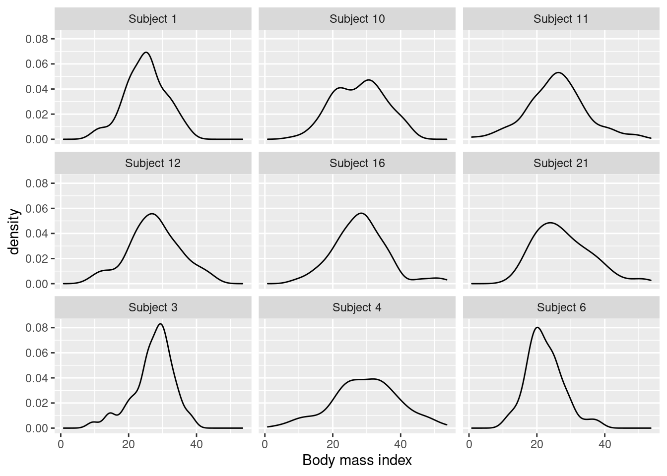
Figure 12.2: Posterior distribution of the missing observations of body mass index in the nhanes2 dataset.
This example has shown how to fit models that can include a simple
imputation mechanism for missing values in the covariates. In order
to obtain estimates of the parameters of the full model, the fit models
obtained in the INLA within MCMC run must be put together with
function inla.merge().
nhanes2.models <- lapply(inlamh.res$model.sim, function(X) { X$model })
nhanes2.imp <- inla.merge(nhanes2.models, rep(1, length(nhanes2.models)))
summary(nhanes2.imp)
##
## Call:
## "inla(formula = chl ~ 1 + bmi + age, data = data)"
## Time used:
## Pre = 86.5, Running = 8.23, Post = 5.34, Total = 100
## Fixed effects:
## mean sd
## (Intercept) 41.953 63.724
## bmi 4.929 2.238
## age40-59 29.421 17.994
## age60-99 49.389 23.081
##
## Model hyperparameters:
## mean sd
## Precision for the Gaussian observations 0.001 0.001
##
## Marginal log-Likelihood: -90.54As compared to the model fit to the observations without missing values of
bmi, the posterior means of all the fixed effects change. The uncertainty
about the intercept and coefficient of bmi also increases (i.e., they have a
larger posterior standard deviation). Note that this may be due to the vague
prior given to the missing values of bmi. However, the uncertainty about the
estimates of age are very close to those obtained with the previous model.
12.6 Final remarks
Although the analysis of data with missing observations is feasible with INLA
it is computationally very expensive when missing values are in the covariates.
Computing the predictive distribution of missing observations in the response
is still reasonable because it is implemented inside the INLA package, but
when different models need to be fit to impute missing observations in the
covariate computational times increase. This may be alleviated by the use of
parallel computing methods and hardware.
Finally, Gómez-Rubio, Cameletti, and Blangiardo (2019) describe a promising approach to include new latent
effects in the model to impute missing observations in the covariates.
References
Buuren, Stef van. 2018. Flexible Imputation of Missing Data. 2nd ed. Boca Raton, FL: CRC Press.
Cameletti, Michela, Virgilio Gómez-Rubio, and Marta Blangiardo. 2019. “Bayesian Modelling for Spatially Misaligned Health and Air Pollution Data Through the INLA-SPDE Approach.” Spatial Statistics 31: 100353. https://doi.org/https://doi.org/10.1016/j.spasta.2019.04.001.
Gómez-Rubio, Virgilio, Michela Cameletti, and Marta Blangiardo. 2019. “Missing Data Analysis and Imputation via Latent Gaussian Markov Random Fields.” arXiv E-Prints, December, arXiv:1912.10981. http://arxiv.org/abs/1912.10981.
Gómez-Rubio, Virgilio, and HRue. 2018. “Markov Chain Monte Carlo with the Integrated Nested Laplace Approximation.” Statistics and Computing 28 (5): 1033–51.
Hoeting, Jennifer, David Madigan, Adrian Raftery, and Chris Volinsky. 1999. “Bayesian Model Averaging: A Tutorial.” Statistical Science 14: 382–401.
Little, Roderick J. A., and Donald B. Rubin. 2002. Statistical Analysis with Missing Data. 2nd ed. New York: Wiley & Sonc, Inc.
Schafer, J. L. 1997. Analysis of Incomplete Multivariate Data. London: Chapman & Hall.
Schonbeck, Y., H. Talma, P. van Dommelen, B. Bakker, S. E. Buitendijk, R. A. Hirasing, and S. van Buuren. 2013. “The World’s Tallest Nation Has Stopped Growing Taller: The Height of Dutch Children from 1955 to 2009.” Pediatric Research 73 (3): 371–77.
Schonbeck, Y., H. Talma, P. van Dommelen, B. Bakker, S. E. Buitendijk, R. A. Hirasing, and S. van Buuren. 2011. “Increase in Prevalence of Overweight in Dutch Children and Adolescents: A Comparison of Nationwide Growth Studies in 1980, 1997 and 2009.” PLoS ONE 6 (11): e27608.
van Buuren, Stef, and Karin Groothuis-Oudshoorn. 2011. “mice: Multivariate Imputation by Chained Equations in R.” Journal of Statistical Software 45 (3): 1–67. https://www.jstatsoft.org/v45/i03/.