Chapter 4 Multilevel Models

4.1 Introduction

Multilevel models (Goldstein 2003) tackle the analysis of data that have been collected from experiments with a complex design. For example, multilevel models are typically used to analyze data from the students’ performance at different tests. Performance is supposed to depend on a number of variables measured at different levels, such as the student, class, school, etc. Nesting occurs because some students will belong to the same class, several classes will belong to the same school and so on. Although the effect of the class or the school is seldom the primary object of study, its effect should be taken into account as it often has an impact on the students’ performance. Hence, class, school, etc. are often modeled using random effects with a complex structure.

A typical problem in multilevel modeling is assessing the variances of the different group effects. For example, is performance among the students in the same class uniform? This can be determined by inspecting the variance estimates of the students’ error terms in a linear mixed-effects model. In addition to the grouped or nested random effects, multilevel data may contain values of the covariates (usually introduced as fixed effects in the model) at different levels. For example, in the case of measuring students’ performance, socio-economic information about the students is available at the individual level, as well as information about the class (size, course, etc.), school, region, etc. These additional data have also an implicit nested or hierarchical structure in different levels that will be included in the model.

Packages nlme (Pinheiro et al. 2018) and lme4 (Bates et al. 2015) provide functions to fit mixed-effects models with complex structure, as well as numerous datasets and examples. Andrew Gelman and Hill (2006) provide an introduction to modeling multilevel data and hierarchical models, and provide a wealth of examples in R. The multilevel package (Bliese 2016) provides a number of datasets with examples and a manual on how to fit multilevel models with R. Faraway (2006) also provides an excellent description of mixed-effects models and provides a good number of examples with R. Some of the examples in this chapter have also been discussed in J. J. Faraway (2019b) and J. J. Faraway (2019a).

4.2 Multilevel models with random effects

The first example will tackle the analysis of the penicillin dataset (Box, Hunter, and Hunter 1978), which is available in the faraway package (Faraway 2016). This dataset measures the production of penicillin depending on the process for production and the blend used. These variables in the data are described in Table 4.1. The penicillin dataset can be loaded and summarized as follows:

library("faraway")
data(penicillin)
summary(penicillin)

##  treat    blend       yield   
##  A:5   Blend1:4   Min.   :77  
##  B:5   Blend2:4   1st Qu.:81  
##  C:5   Blend3:4   Median :87  
##  D:5   Blend4:4   Mean   :86  
##        Blend5:4   3rd Qu.:89  
##                   Max.   :97

Table 4.1: Summary of variables in the penicillin dataset in the faraway package.

Variable	Description
yield	Production of penicillin.
treat	Production type (factor with 4 levels).
blend	Blend used for production (factor with 5 levels).

Figure 4.1 displays the data and shows the effect of the different production methods and blend.

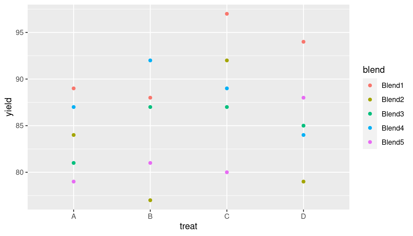
Figure 4.1: Penicillin production on production method (treat) and blend (blend).

In this analysis, the interest is on how the production method (treat) affects the production of penicillin. However, production methods use a raw material (corn steep liquor) which is quite variable and may affect the production. Furthermore, this is produced in blends that are only enough for four runs of the production of penicillin. Hence, there is the risk that an observed increment in the production may be due to the actual blend used and not the production method and it is required to account for the blend in the model even if it is not of interest.

Hence, treat will be introduced in the model as a fixed effect and blend will be introduced in the model as a random effect. Note that the four runs coming from the same blend will share the same value of the random effect. Hence, each observation of production of penicillin can be regarded as being in a level of the model, with each one of the four production types in level 2 of the model.

The model can be written down as:

\[ \texttt{yield}_{ij} = \beta_i \texttt{treat}_i + u_j + e_{ij};\ i=1,\ldots, 4,\ j=1\ldots, 5 \]

\[ u_j \sim N(0, \tau_u);\ j=1\ldots, 5 \]

Altogether, there are 20 observations. Note that we have not included an intercept in the model because we aim at estimating the different effects of the treatments directly.

Note that the term \(u_j\) is sometimes referred to as a random intercept as it is a random effect and it is the same for the same level of the blend variable, acting similarly as an intercept for the observations in that group alone. Also, the prior on the precision of the random effects \(\tau_u\) is set to a Gamma distribution with parameters \(0.001\) and \(0.001\) as this is a commonly used vague prior. However, see Chapter 5 and, in particular, A Gelman (2006) and Andrew Gelman and Hill (2006), Chapter 19, for a general discussion on priors for the precisions of the random effects and alternatives to the prior Gamma distribution.

The Gamma prior with parameters \(0.001\) and \(0.001\) can be set beforehand and used later in the definition of the latent random effects:

# Set prior on precision
prec.prior <- list(prec = list(param = c(0.001, 0.001)))

Before the analysis, the reference level of the production type will be set to D so that our results can be compared to those in Faraway (2006):

penicillin$treat <- relevel(penicillin$treat, "D")

The mixed-effects model can be fit with INLA as follows:

library("INLA")
inla.pen <- inla(yield ~ 1 + treat + f(blend, model = "iid",
    hyper = prec.prior),
  data = penicillin, control.predictor = list(compute = TRUE))
summary(inla.pen)

## 
## Call:
##    c("inla(formula = yield ~ 1 + treat + f(blend, model = \"iid\", 
##    hyper = prec.prior), ", " data = penicillin, control.predictor = 
##    list(compute = TRUE))" ) 
## Time used:
##     Pre = 0.667, Running = 0.157, Post = 0.0356, Total = 0.859 
## Fixed effects:
##               mean    sd 0.025quant 0.5quant 0.975quant   mode   kld
## (Intercept) 86.000 2.713     80.622   86.000     91.382 86.000 0.001
## treatA      -1.991 2.905     -7.784   -1.992      3.795 -1.993 0.000
## treatB      -0.996 2.905     -6.789   -0.996      4.789 -0.997 0.000
## treatC       2.987 2.905     -2.810    2.988      8.769  2.990 0.000
## 
## Random effects:
##   Name     Model
##     blend IID model
## 
## Model hyperparameters:
##                                          mean    sd 0.025quant 0.5quant
## Precision for the Gaussian observations 0.062 0.023      0.027    0.059
## Precision for blend                     0.126 0.160      0.011    0.078
##                                         0.975quant  mode
## Precision for the Gaussian observations      0.117 0.053
## Precision for blend                          0.535 0.030
## 
## Expected number of effective parameters(stdev): 6.13(1.31)
## Number of equivalent replicates : 3.26 
## 
## Marginal log-Likelihood:  -84.20 
## Posterior marginals for the linear predictor and
##  the fitted values are computed

In addition to the summary of the model fit above, Figure 4.2 shows the posterior marginals of the latent effects and hyperparameters in the model.

For comparison purposes, the same model has been fitted with function lmer() from package lme4 using restricted maximum likelihood:

library("lme4")
lmer.pen <- lmer(yield ~ 1 + treat + (1|blend), data = penicillin)
summary(lmer.pen)

## Linear mixed model fit by REML ['lmerMod']
## Formula: yield ~ 1 + treat + (1 | blend)
##    Data: penicillin
## 
## REML criterion at convergence: 103.8
## 
## Scaled residuals: 
##    Min     1Q Median     3Q    Max 
## -1.415 -0.502 -0.164  0.683  1.284 
## 
## Random effects:
##  Groups   Name        Variance Std.Dev.
##  blend    (Intercept) 11.8     3.43    
##  Residual             18.8     4.34    
## Number of obs: 20, groups:  blend, 5
## 
## Fixed effects:
##             Estimate Std. Error t value
## (Intercept)    86.00       2.48   34.75
## treatA         -2.00       2.75   -0.73
## treatB         -1.00       2.75   -0.36
## treatC          3.00       2.75    1.09
## 
## Correlation of Fixed Effects:
##        (Intr) treatA treatB
## treatA -0.555              
## treatB -0.555  0.500       
## treatC -0.555  0.500  0.500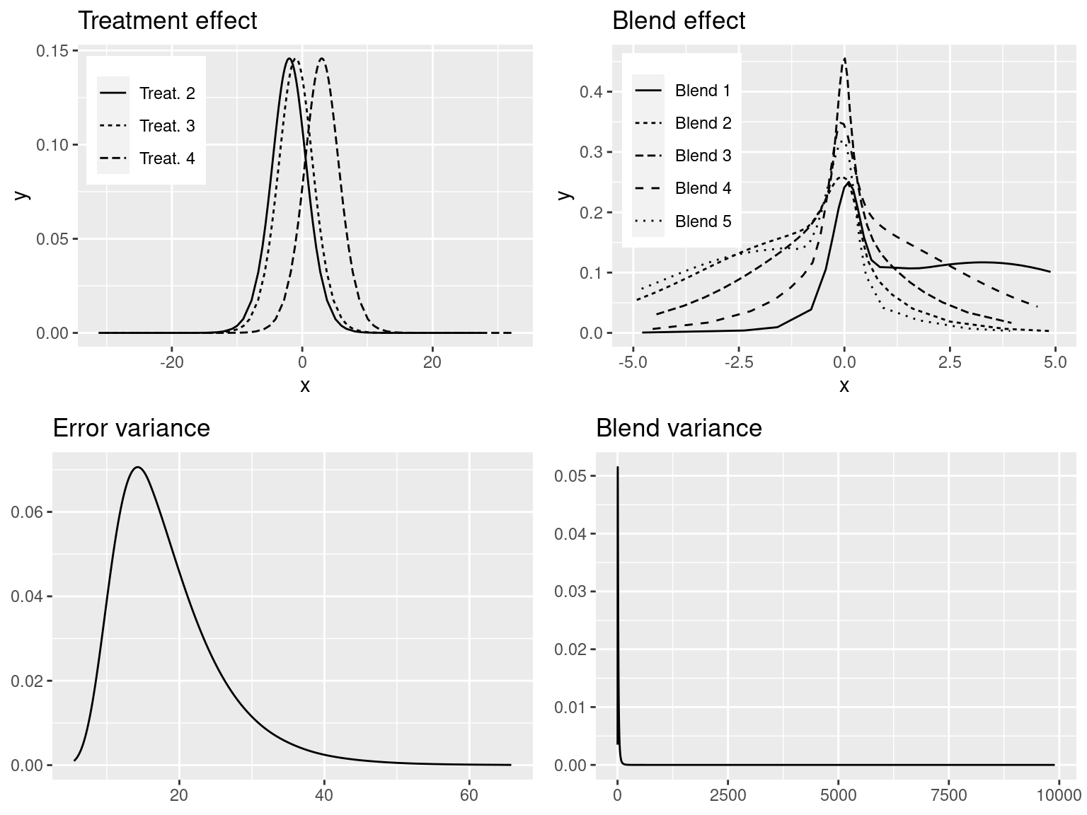

Figure 4.2: Marginals of fixed effects of the production method (top-left), blend random-effects (top-right), variance of the error term (bottom-left) and variance of the blend effect (bottom-right).

The main differences lie between the estimates of the variances of the random effects and the error term. As suggested in J. J. Faraway (2019b), a more informative prior on the precision of the blend random effects would be required here.

Alternatively, this model can be fit using the latent effect z, which requires a matrix of random effects. Although this is a rather simple model that can be easily fit with the iid latent effect, we will develop an example in order to show how the matrix of random effects can be obtained with function model.matrix().

Function model.matrix() is usually employed to obtain the design matrix for linear models from a model formula and a dataset. It has the nice feature of expanding factors as dummy variables, which is what is needed to create a design matrix for the random effects. The resulting matrix is likely to be very sparse, so it makes sense to convert it into a Matrix (Bates and Maechler 2019) to obtain a sparse representation.

The creation of the design matrix of the random effects can be as follows:

Z <- as(model.matrix(~ 0 + blend, data = penicillin), "Matrix")

Figure 4.3 shows the structure of the matrix created. Shaded elements are equal to 1 and all the other elements are zero. Note that this matrix is used to map the group-level random effects in the linear predictor of the observations.

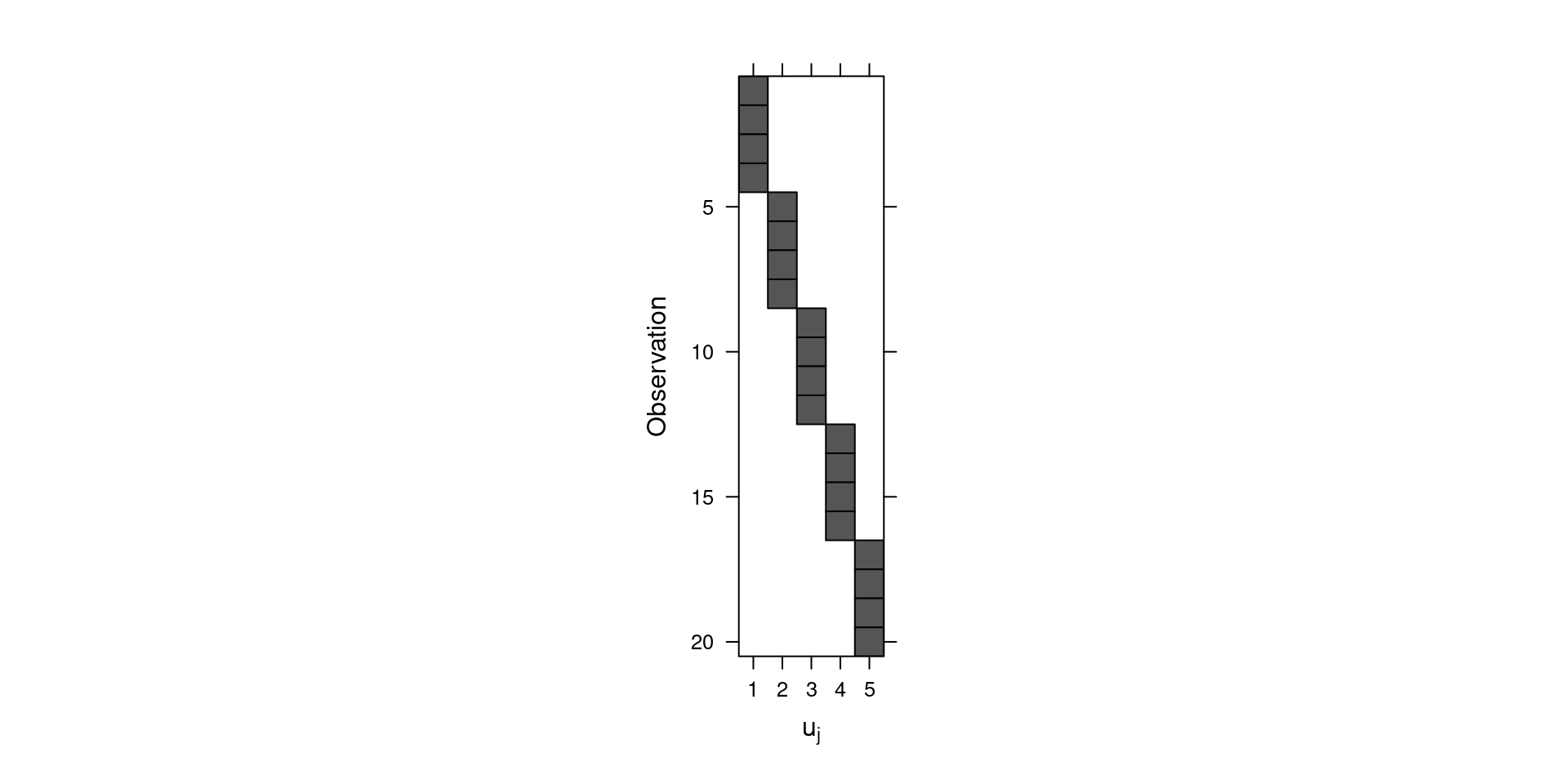
Figure 4.3: Representation of the design matrix of the random effects.

Once the matrix has been created, then a new index is needed (for random effect z) and the model can be fitted:

penicillin$ID <- 1:nrow(penicillin)

inla.pen.z <- inla(yield ~ 1 + treat +  f(ID, model = "z", Z = Z,
  hyper = list(prec = list(param = c(0.001, 0.001)))),
  data = penicillin, control.predictor = list(compute = TRUE))
summary(inla.pen.z)

## 
## Call:
##    c("inla(formula = yield ~ 1 + treat + f(ID, model = \"z\", Z = Z, 
##    ", " hyper = list(prec = list(param = c(0.001, 0.001)))), data = 
##    penicillin, ", " control.predictor = list(compute = TRUE))") 
## Time used:
##     Pre = 0.264, Running = 0.274, Post = 0.0258, Total = 0.564 
## Fixed effects:
##               mean    sd 0.025quant 0.5quant 0.975quant   mode kld
## (Intercept) 86.000 2.715     80.627   86.000     91.372 86.000   0
## treatA      -1.991 2.940     -7.856   -1.992      3.867 -1.993   0
## treatB      -0.996 2.940     -6.861   -0.996      4.862 -0.997   0
## treatC       2.987 2.940     -2.883    2.988      8.841  2.990   0
## 
## Random effects:
##   Name     Model
##     ID Z model
## 
## Model hyperparameters:
##                                          mean    sd 0.025quant 0.5quant
## Precision for the Gaussian observations 0.062 0.024      0.027    0.059
## Precision for ID                        0.158 0.244      0.012    0.086
##                                         0.975quant  mode
## Precision for the Gaussian observations      0.118 0.052
## Precision for ID                             0.743 0.030
## 
## Expected number of effective parameters(stdev): 6.00(1.38)
## Number of equivalent replicates : 3.33 
## 
## Marginal log-Likelihood:  -84.11 
## Posterior marginals for the linear predictor and
##  the fitted values are computed

The main difference between the iid and z latent effects is that the first one will produce exactly as many random effects as defined in the model. On the other hand, the z model will produce as many random effects as data, which are the random effects of the groups plus some tiny error. This is defined by the precision parameter when the latent effect is defined using the f() function. See Chapter 3 for details.

When the z model is used, INLA will report summary statistics on the subject-level random effects followed by the group-level random effects. As mentioned above, subject-level random effects are the corresponding group-level random effects plus some tiny noise that is required for model fitting. In this particular case, there are 20 observations, with 5 groups to define the random effects. Hence, the number of rows in inla.pen.z$summary.random$ID is 25.

Figure 4.4 shows the posterior means of the random effects obtained with the iid and the z model. In general, the agreement between the estimates from both models is quite good.

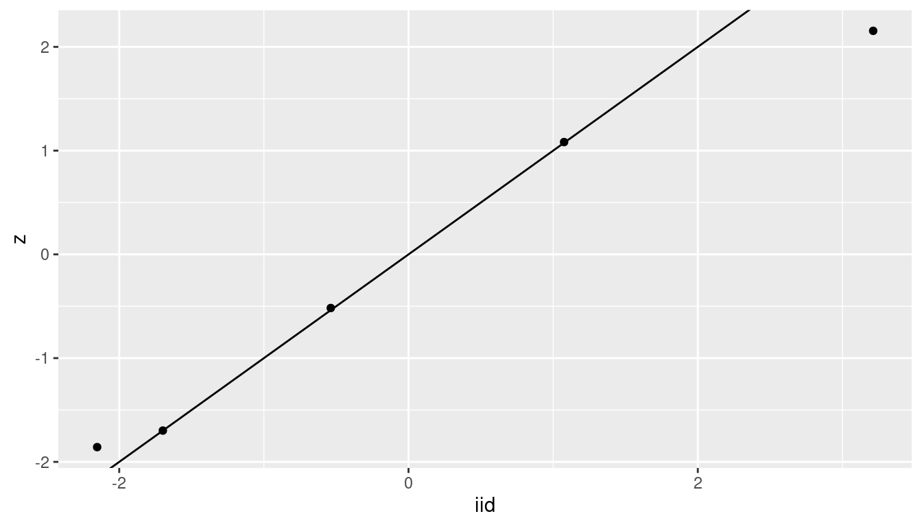
Figure 4.4: Multilevel models fitted with iid and z random effects.

4.3 Multilevel models with nested effects

The eggs dataset (Bliss 1967) in the faraway package contains data on fat content in different samples of egg powder. The analyzes were carried out at different laboratories, by different technicians. Also, each sample was split into two parts that were analyzed separately by the same technician.

A summary of the variables in the dataset is in Table 4.2, which is loaded and summarized as follows:

data(eggs)

summary(eggs)

##       Fat         Lab    Technician Sample
##  Min.   :0.060   I  :8   one:24     G:24  
##  1st Qu.:0.307   II :8   two:24     H:24  
##  Median :0.370   III:8                    
##  Mean   :0.388   IV :8                    
##  3rd Qu.:0.430   V  :8                    
##  Max.   :0.800   VI :8

This is a typical example of nested random effects because the technicians are nested within laboratories, so their ids cannot be directly used when defining the random effects as this will consider technician one in laboratory I to be the same as technician one in laboratory II and so on. Hence, using the technician ids directly will make the effect of technician one in lab I to be the same as technician one in lab II, etc. Nesting of the random effects can be taken into account by simply creating a new index variable that accounts for the technician and the laboratory.

Table 4.2: Summary of the variables in the eggs dataset.

Variable	Description
Fat	Fat content.
Lab	Laboratory id (a factor from I to VI).
Technician	Technician id (a factor of one or two).
Sample	Sample id (a factor of G or H).

The model to be fitted now is:

\[ \textrm{fat}_{ijkl} = \beta_0 + \textrm{lab}_{i} + \textrm{technician}_{j:i} + \textrm{sample}_{k:(j:i)} + \varepsilon_{ijkl}, i = 1, \ldots, 6; j = 1, 2; k = 1,2; l = 1,2 \]

\[ \varepsilon_{ijkl} \sim N(0, \tau) \]

\[ \textrm{lab}_{i} \sim N(0, \tau_{lab}), i = 1, \ldots, 4 \]

\[ \textrm{technician}_{j:i} \sim N(0, \tau_{tec}), j:i = 1, \ldots, 12 \]

\[ \textrm{sample}_{k:(j:i)} \sim N(0, \tau_{sam}), k:(j:i) = 1, \ldots, 24 \]

Indices are defined for laboratory (\(i\)), technician (\(j\)), samples (\(k\)) and half-sample (\(l\)). Index \(j:i\) denotes that technician is nested within a laboratory and, similarly, index \(k:(j:i)\) denotes nesting of samples within technicians (who are themselves nested within laboratories).

Similarly as in the previous example, function model.matrix() can be used with a formula that includes the nesting of the variable to create the matrices of the random effects:

Zlt <- as(model.matrix( ~ 0 + Lab:Technician, data = eggs), "Matrix")
Zlts <- as(model.matrix( ~ 0 + Lab:Technician:Sample, data = eggs), "Matrix")

Figure 4.5 shows the matrices created. Note how the non-zero elements appear in different ways in each matrix. For the nested random effect of the technician, the non-zero elements appear in groups of four, since each technician examined two samples (which were in turn split in two). For the nested random effect on Sample, these appear in groups of two as each sample was split in two and analyzed.

Note that now there are two nested random effects. The first one is the technician, which is nested within a laboratory, and the second one is the sample, which is analyzed by different technicians from different laboratories.

Before model fitting, two indices for the nested random effects must be created:

# Index for techinician
eggs$IDt <- 1:nrow(eggs)
# Index for technician:sample
eggs$IDts <- 1:nrow(eggs)

Figure 4.5: Representation of the design matrix of the random effects for the eggs dataset.

The final model contains a non-nested random effect for the laboratory (which is iid) plus the two nested random effects:

inla.eggs <- inla(Fat ~ 1 + f(Lab, model = "iid", hyper = prec.prior) +
    f(IDt, model = "z", Z = Zlt, hyper = prec.prior) +
    f(IDts, model = "z", Z = Zlts, hyper = prec.prior),
  data = eggs, control.predictor = list(compute = TRUE))

summary(inla.eggs)

## 
## Call:
##    c("inla(formula = Fat ~ 1 + f(Lab, model = \"iid\", hyper = 
##    prec.prior) + ", " f(IDt, model = \"z\", Z = Zlt, hyper = 
##    prec.prior) + f(IDts, ", " model = \"z\", Z = Zlts, hyper = 
##    prec.prior), data = eggs, ", " control.predictor = list(compute = 
##    TRUE))") 
## Time used:
##     Pre = 0.312, Running = 0.229, Post = 0.0292, Total = 0.57 
## Fixed effects:
##              mean    sd 0.025quant 0.5quant 0.975quant  mode kld
## (Intercept) 0.387 0.056      0.275    0.387        0.5 0.387   0
## 
## Random effects:
##   Name     Model
##     Lab IID model
##    IDt Z model
##    IDts Z model
## 
## Model hyperparameters:
##                                           mean     sd 0.025quant 0.5quant
## Precision for the Gaussian observations 154.22  41.86      86.16   149.69
## Precision for Lab                       360.88 661.86      22.49   176.20
## Precision for IDt                       207.99 216.22      28.23   144.07
## Precision for IDts                      347.77 297.79      62.45   263.94
##                                         0.975quant   mode
## Precision for the Gaussian observations     249.25 141.05
## Precision for Lab                          1854.37  56.24
## Precision for IDt                           776.12  71.67
## Precision for IDts                         1131.99 153.83
## 
## Expected number of effective parameters(stdev): 16.87(2.58)
## Number of equivalent replicates : 2.85 
## 
## Marginal log-Likelihood:  7.73 
## Posterior marginals for the linear predictor and
##  the fitted values are computed

Alternatively, an index variable can be created from the matrices of the random effects to be used with the iid random effect, as follows:

eggs$labtech <- as.factor(apply(Zlt, 1, function(x){names(x)[x == 1]}))
eggs$labtechsamp <- as.factor(apply(Zlts, 1, function(x){names(x)[x == 1]}))

Then, the model can be fit as follows:

inla.eggs.iid <- inla(Fat ~ 1 + f(Lab, model = "iid", hyper = prec.prior) +
    f(labtech, model = "iid", hyper = prec.prior) +
    f(labtechsamp, model = "iid", hyper = prec.prior),
  data = eggs, control.predictor = list(compute = TRUE))

summary(inla.eggs.iid)

## 
## Call:
##    c("inla(formula = Fat ~ 1 + f(Lab, model = \"iid\", hyper = 
##    prec.prior) + ", " f(labtech, model = \"iid\", hyper = prec.prior) 
##    + f(labtechsamp, ", " model = \"iid\", hyper = prec.prior), data = 
##    eggs, control.predictor = list(compute = TRUE))" ) 
## Time used:
##     Pre = 0.295, Running = 0.135, Post = 0.0274, Total = 0.458 
## Fixed effects:
##              mean    sd 0.025quant 0.5quant 0.975quant  mode kld
## (Intercept) 0.387 0.056      0.275    0.387        0.5 0.387   0
## 
## Random effects:
##   Name     Model
##     Lab IID model
##    labtech IID model
##    labtechsamp IID model
## 
## Model hyperparameters:
##                                           mean     sd 0.025quant 0.5quant
## Precision for the Gaussian observations 154.09  41.79      86.12   149.58
## Precision for Lab                       360.89 661.86      22.49   176.20
## Precision for labtech                   208.18 216.60      28.24   144.14
## Precision for labtechsamp               347.80 297.79      62.53   263.97
##                                         0.975quant   mode
## Precision for the Gaussian observations     248.95 140.97
## Precision for Lab                          1854.36  56.24
## Precision for labtech                       777.28  71.67
## Precision for labtechsamp                  1131.89 153.91
## 
## Expected number of effective parameters(stdev): 16.85(2.58)
## Number of equivalent replicates : 2.85 
## 
## Marginal log-Likelihood:  7.73 
## Posterior marginals for the linear predictor and
##  the fitted values are computed

Note how both ways of fitting the model provide very similar estimates. The fact that some estimates of the precision are that high may indicate that these parameters are poorly identified in the model and may require the use of less vague priors.

It is important to mention that some of the estimates of the precisions are quite high and narrow, and it might be better to have a more informative prior on these precisions (J. J. Faraway 2019b).

4.4 Multilevel models with complex structure

Multilevel models have traditionally been associated with education research on measuring students’ performance. See, for example, Goldstein (2003) and the references therein. This type of research often creates rich datasets with data available at different levels: student, class, school, etc. Both covariates and a nesting structure are available for the design of mixed-effects models.

Carpenter, Goldstein, and Kenward (2011) describe a multilevel model to analyze the performance of children using literacy and numeracy scores. This is a subset of the original dataset, which is fully described in Blatchford et al. (2002). The study aimed at measuring the effect of class size on children in their first full year of education. For this reason, literacy and numeracy scores are available at school entry and at the end of the first year of school for each student, in addition to the class size. Table 4.3 shows the variables included in this dataset.

Table 4.3: Summary of the variables in the analysis of school performance in children (Carpenter, Goldstein, and Kenward 2011).

Variable	Description
clsnr	Class identifier.
pupil	Student identifier.
nlitpost	Standardized literacy score at the end of 1st school year
nmatpost	Standardized numeracy score at the end of 1st school year
nlitpre	Standardized literacy score at school entry
nmatpre	Standardized numeracy score at school entry
csize	Class size (as a factor with four levels)

The following code can be used to load the data into R. Note that the code includes some lines to handle missing values (coded as -9.9990e+029) and label the categories of class size into four groups.

#Read data
csize_data <- read.csv (file = "data/class_size_data.txt", header = FALSE,
  sep = "", dec = ".")

#Set names
names(csize_data) <- c("clsnr", "pupil", "nlitpre", "nmatpre", "nlitpost",
  "nmatpost", "csize")

#Set NA's
csize_data [csize_data < -1e+29 ] <- NA

#Set class size levels
csize_data$csize <- as.factor(csize_data$csize)
levels(csize_data$csize) <- c("<=19", "20-24", "25-29", ">=30")

summary(csize_data)

##      clsnr         pupil         nlitpre        nmatpre     
##  Min.   :  1   Min.   :   1   Min.   :-3.7   Min.   :-2.89  
##  1st Qu.: 84   1st Qu.:1849   1st Qu.:-0.6   1st Qu.:-0.62  
##  Median :170   Median :3698   Median : 0.0   Median :-0.08  
##  Mean   :174   Mean   :3698   Mean   : 0.0   Mean   :-0.01  
##  3rd Qu.:262   3rd Qu.:5546   3rd Qu.: 0.7   3rd Qu.: 0.68  
##  Max.   :400   Max.   :7394   Max.   : 3.4   Max.   : 1.88  
##                               NA's   :766    NA's   :302    
##     nlitpost       nmatpost      csize     
##  Min.   :-2.8   Min.   :-3.1   <=19 : 301  
##  1st Qu.:-0.7   1st Qu.:-0.7   20-24:1401  
##  Median : 0.0   Median : 0.0   25-29:3484  
##  Mean   : 0.0   Mean   : 0.0   >=30 :1520  
##  3rd Qu.: 0.6   3rd Qu.: 0.7   NA's : 688  
##  Max.   : 2.7   Max.   : 2.8               
##  NA's   :1450   NA's   :1409

The dataset contains a number of missing values because the aim of Carpenter, Goldstein, and Kenward (2011) was to deal with missing data in the study and impute them. However, we will consider here children with complete observations only, and focus on the numeracy score only, which is also discussed in the original paper.

Hence, the next step is to keep the rows with full observations in all variables (but nlitpost, which will be ignored for now):

csize_data2 <- na.omit(csize_data[, -5])

Note that this makes the dataset have 5033 rows instead of the original 7394. For now, we will forget about the observations with missing data but this is something that should be taken into account in the analysis at some point (see Chapter 12).

Carpenter, Goldstein, and Kenward (2011) are interested in modeling the literacy and numeracy scores at the end of the first year of school on other variables, with particular interest in school size. Note that all the other variables have been measured at the student level and this makes this dataset multilevel. Note that now students are nested within classes. Furthermore, for this initial analysis the response variable will be nmatpost.

Following Carpenter, Goldstein, and Kenward (2011), the multilevel model fitted now is:

\[ \textrm{nmatpost}_{ij} = \beta_{0ij} + \beta_1 \textrm{nmatpre}_{ij} + \beta_2 \textrm{nlitpre}_{ij} + \beta_3 \textrm{csize}_{ij}^{\textrm{20-24}} + \beta_4 \textrm{csize}_{ij}^{\textrm{25-29}} + \beta_5 \textrm{csize}_{ij}^{\textrm{>=30}} \]

\[ \beta_{0ij} = \beta_0 + u_j + \varepsilon_{ij} \]

\[ u_j \sim N(0,\tau_u);\ \varepsilon_{ij}\sim N(0, \tau); i=1,\ldots,n_j;\ j=1,\ldots,n_c \]

Here, \(\beta_{0ij}\) represents a random term on the student, which comprises an overall intercept \(\beta_0\), a class random effect \(u_j\) and a student random effect \(\varepsilon_{ij}\) (which is in fact modeled by the error of the Gaussian likelihood). Variable \(\textrm{csize}_{ij}^{\textrm{20-24}}\) is a dummy variable that is 1 if the class size is “20-24” and 0 otherwise. \(\textrm{csize}_{ij}^{\textrm{25-29}}\) and \(\textrm{csize}_{ij}^{\textrm{>=30}}\) are defined analogously. The total number of classes is denoted by \(n_c\) and the number of students in class \(j\) by \(n_j\).

The model can be summarized as students being in level 1 in the model, with student level numeracy and literacy scores and an associated error (or random effect) \(\varepsilon_{ij}\). The next layer in the model, level 2, is about the class, for which covariate class size and a class-level random effect \(u_j\) is included. This multilevel model can be easily fitted with INLA:

inla.csize <- inla(nmatpost ~ 1 + nmatpre + nlitpre + csize +
  f(clsnr, model = "iid"), data = csize_data2)

summary(inla.csize)

## 
## Call:
##    c("inla(formula = nmatpost ~ 1 + nmatpre + nlitpre + csize + 
##    f(clsnr, ", " model = \"iid\"), data = csize_data2)") 
## Time used:
##     Pre = 0.3, Running = 2.22, Post = 0.0284, Total = 2.55 
## Fixed effects:
##               mean    sd 0.025quant 0.5quant 0.975quant   mode kld
## (Intercept)  0.270 0.141     -0.008    0.270      0.547  0.270   0
## nmatpre      0.367 0.015      0.337    0.367      0.397  0.367   0
## nlitpre      0.372 0.015      0.343    0.372      0.402  0.372   0
## csize20-24  -0.114 0.157     -0.422   -0.114      0.193 -0.115   0
## csize25-29  -0.319 0.149     -0.611   -0.319     -0.026 -0.319   0
## csize>=30   -0.340 0.160     -0.654   -0.340     -0.026 -0.340   0
## 
## Random effects:
##   Name     Model
##     clsnr IID model
## 
## Model hyperparameters:
##                                         mean    sd 0.025quant 0.5quant
## Precision for the Gaussian observations 2.67 0.055       2.56     2.67
## Precision for clsnr                     4.02 0.397       3.28     4.01
##                                         0.975quant mode
## Precision for the Gaussian observations       2.77 2.67
## Precision for clsnr                           4.84 4.01
## 
## Expected number of effective parameters(stdev): 232.34(2.02)
## Number of equivalent replicates : 21.66 
## 
## Marginal log-Likelihood:  -5051.96

Point estimates of the model are very similar to those obtained using restricted maximum likelihood as reported in Carpenter, Goldstein, and Kenward (2011).

Regarding the effect of class size on the numeracy score at the end of the first school year, it seems that this is reduced with the increase of the class size. Furthermore, variation between students is larger than between classes.

4.5 Multilevel models for longitudinal data

Belenky et al. (2003) describe a study of reaction time in patients under sleep deprivation up to 10 days. This dataset is available in package lme4 as dataset sleepstudy. See also Jovanovic (2015) for an analysis of this dataset with R using different methods.

Table 4.4: Summary of variables in the sleepstudy dataset in package lme4.

Variable	Description
Reaction	Average reaction time (in ms).
Days	Number of days in sleep deprivation.
Subject	Subject id in the study.

Table 4.4 shows the variables in the dataset, which can be loaded as follows:

library("lme4")
data(sleepstudy)

Reaction time will be rescaled by dividing by 1000 to have the reaction time in seconds as this makes estimation with INLA more stable:

#Scale Reaction
sleepstudy$Reaction <- sleepstudy$Reaction / 1000

Then, the resulting dataset can be summarized as:

summary(sleepstudy)

##     Reaction          Days        Subject   
##  Min.   :0.194   Min.   :0.0   308    : 10  
##  1st Qu.:0.255   1st Qu.:2.0   309    : 10  
##  Median :0.289   Median :4.5   310    : 10  
##  Mean   :0.298   Mean   :4.5   330    : 10  
##  3rd Qu.:0.337   3rd Qu.:7.0   331    : 10  
##  Max.   :0.466   Max.   :9.0   332    : 10  
##                                (Other):120

The analysis of this dataset is interesting because time deprivation seems to affect subjects’ reaction time differently. This effect is shown in Figure 4.6. Hence, this is an interesting dataset for a longitudinal model.

In order to fit a reasonable model to the data we need to allow for different slopes for variable Days for different subjects in the study. This is often achieved by including a random coefficient in the model. This means that each subject will have an associated random effect that multiplies the value of the covariate and that will produce a different linear trend for each patient.

First of all, a mixed effects model with a fixed effect on Days and a random effect on Subject is fit. This model assumes the same slope of the effect of Days on the students.

inla.sleep <- inla(Reaction ~ 1 + Days + f(Subject, model = "iid"),
  data = sleepstudy)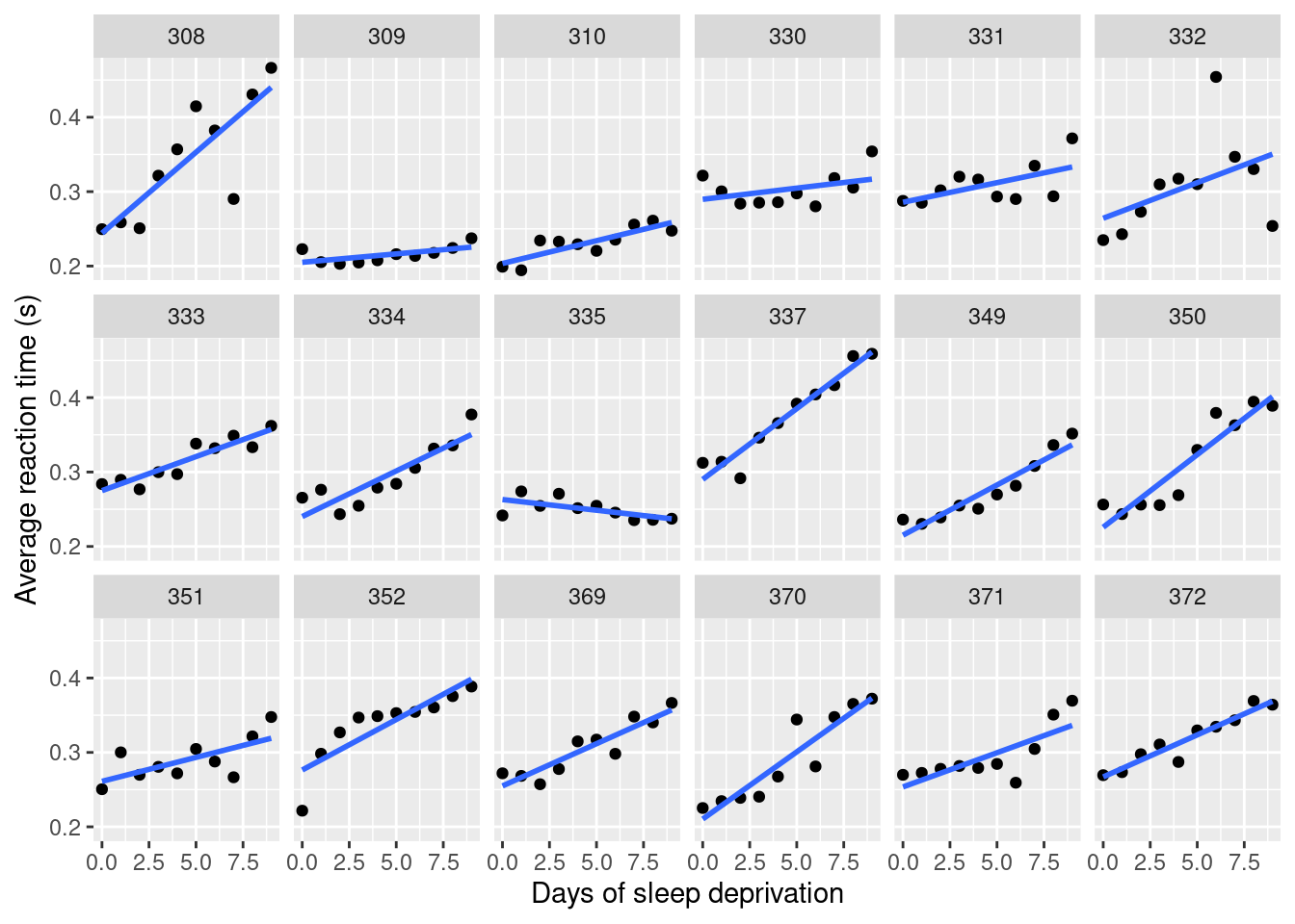

Figure 4.6: Effect of time (in days) of sleep deprivation on reaction time from the `sleepstudy’ dataset.

summary(inla.sleep)

## 
## Call:
##    c("inla(formula = Reaction ~ 1 + Days + f(Subject, model = 
##    \"iid\"), ", " data = sleepstudy)") 
## Time used:
##     Pre = 0.214, Running = 0.136, Post = 0.0226, Total = 0.373 
## Fixed effects:
##              mean    sd 0.025quant 0.5quant 0.975quant  mode kld
## (Intercept) 0.251 0.010      0.232    0.251      0.271 0.251   0
## Days        0.010 0.001      0.009    0.010      0.012 0.010   0
## 
## Random effects:
##   Name     Model
##     Subject IID model
## 
## Model hyperparameters:
##                                            mean     sd 0.025quant 0.5quant
## Precision for the Gaussian observations 1059.38 118.20     842.33  1054.35
## Precision for Subject                    831.28 296.08     384.05   788.55
##                                         0.975quant    mode
## Precision for the Gaussian observations    1306.77 1046.01
## Precision for Subject                      1532.67  706.17
## 
## Expected number of effective parameters(stdev): 18.79(0.497)
## Number of equivalent replicates : 9.58 
## 
## Marginal log-Likelihood:  324.29

A model with subject-level random slopes on Days can be fitted by including a second term when defining the random effect with the values of the covariates:

inla.sleep.w <- inla(Reaction ~ 1 + f(Subject, Days, model = "iid"),
  data = sleepstudy, control.predictor = list(compute = TRUE))

Note that term f(Subject, Days, model = "iid") now includes two arguments before model. The first one defines the groups (and, hence, the number of random slopes) and the second one is the value of the covariate (which is, in principle, slightly different among subjects). In this case, order matters and the first two arguments cannot be exchanged.

The summary of the model is:

summary(inla.sleep.w)

## 
## Call:
##    c("inla(formula = Reaction ~ 1 + f(Subject, Days, model = 
##    \"iid\"), ", " data = sleepstudy, control.predictor = list(compute 
##    = TRUE))" ) 
## Time used:
##     Pre = 0.215, Running = 0.4, Post = 0.0266, Total = 0.642 
## Fixed effects:
##              mean    sd 0.025quant 0.5quant 0.975quant  mode kld
## (Intercept) 0.255 0.004      0.247    0.255      0.263 0.255   0
## 
## Random effects:
##   Name     Model
##     Subject IID model
## 
## Model hyperparameters:
##                                            mean      sd 0.025quant
## Precision for the Gaussian observations 1205.91  135.16     958.15
## Precision for Subject                   7215.08 2423.91    3447.03
##                                         0.5quant 0.975quant    mode
## Precision for the Gaussian observations  1200.04    1489.36 1190.19
## Precision for Subject                    6900.71   12883.09 6284.39
## 
## Expected number of effective parameters(stdev): 19.76(0.236)
## Number of equivalent replicates : 9.11 
## 
## Marginal log-Likelihood:  336.25 
## Posterior marginals for the linear predictor and
##  the fitted values are computed

Figure 4.7 shows the posterior means of the intercept and random effect (slope) of the fit line on the data using the random slope model (black line) and a line obtained by fitting a linear regression to the data of each subject (in blue).

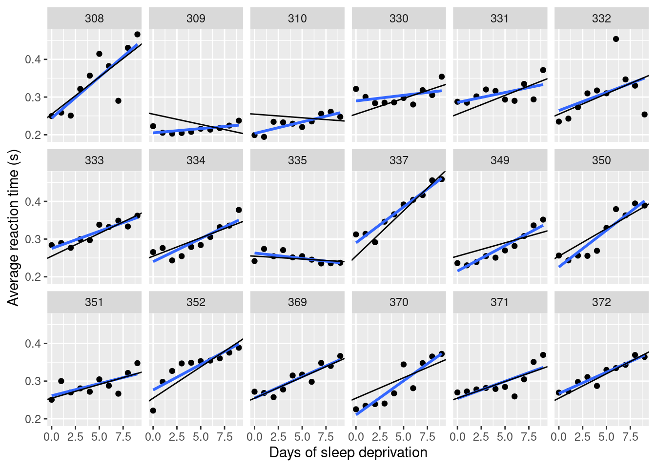
Figure 4.7: Posterior mean of fit line using model with a random slope. The blue line represents a fit line using linear regression and the black line represents the line with the posterior mean of the slope and group effect.

4.6 Multilevel models for binary data

The multilevel models presented in previous sections can be extended to the case of non-Gaussian responses. For the case of binary data, a logistic regression can be proposed with fixed and random effects to account for different levels of variation in the data.

As an example, we will consider data from a survey for the 1988 election in the United States of America. These data have been analyzed in Andrew Gelman and Hill (2006) and it is available from Prof. Gelman’s website (see Preface for details). Note that there are no observations from two states (Alaska and Hawaii) and hence the actual number of states in the data is 49 instead of 51.

This is a subset of a dataset comprising different polls on the 1988 presidential elections in the United States of America and only the latest survey conducted by CBS News will be considered. In this election, the Republican candidate was George H. W. Bush and the Democrat candidate was Michael Dukakis. The variables in this dataset are summarized in Table 4.5.

Table 4.5: Summary of the variables in the dataset on the 1988 US presidential election poll.

Variable	Description
org	Organization that conducted the survey.
year	Year of survey.
survey	Survey id.
bush	Respondent will vote for Bush (1 = yes, 0 = no).
state	State id of respondent (including D.C.).
edu	Education level of respondent.
age	Age category of respondent.
female	Respondent is female.
black	Respondent is black.
weight	Survey weight.

The dataset can be loaded as follows:

election88 <- read.table(file = "data/polls.subset.dat")

Gelman and Little (1997) give more details about the categories of variables age and edu in the dataset and these are used to label the different levels:

election88$age <- as.factor(election88$age)
levels(election88$age) <- c("18-29", "30-44", "45-64", "65+")

election88$edu <- as.factor(election88$edu)
levels(election88$edu) <- c("not.high.school.grad", "high.school.grad",
  "some.college", "college.grad")

The analysis in Andrew Gelman and Hill (2006) also includes a region indicator for each state. The region indicator has been obtained from the files in Prof. Gelman’s website and will be added as a new region column to the original dataset:

# Add region
election88$region <- c(3, 4, 4, 3, 4, 4, 1, 1, 5, 3, 3, 4, 4, 2, 2, 2, 2,
  3, 3, 1, 1, 1, 2, 2, 3, 2, 4, 2, 4, 1, 1, 4, 1, 3, 2, 2, 3, 4, 1, 1, 3,
  2, 3, 3, 4, 1, 3, 4, 1, 2, 4)[as.numeric(election88$state)]

Andrew Gelman and Hill (2006) propose a number of models to analyze this dataset. This is a multilevel dataset because respondents are nested within states, which in turn are nested within regions. In addition, we have individual covariates as well as the indicator of the state, which could be used to include random effects in the model. Here, respondents will be in level one of the model, with state being the second level of the model. Region could be considered a third level of the model.

Hence, a simple approach would be to model the probability of voting for Bush \(\pi_{ij}\) of respondent \(i\) in state \(j\) on gender, race and state (included as a random effect) using a logit link function, as follows:

\[ \logit(\pi_{ij}) = \beta_0 + \beta_1 \textrm{female}_{ij} + \beta_2 \textrm{black}_{ij} + \beta_3 \textrm{age}_{ij}^{30-44} + \beta_4 \textrm{age}_{ij}^{45-64} + \beta_5 \textrm{age}_{ij}^{65+} + \]

\[ \beta_6 \textrm{edu}_{ij}^{high.school.grad} + \beta_7 \textrm{edu}_{ij}^{some.college} + \beta_8 \textrm{edu}_{ij}^{college.grad} + u_j;\ i=1,\ldots,n_j;\ j = 1, \ldots, 51 \]

\[ u_j \sim N(0, \tau_u);\ j = 1, \ldots, 51 \]

Note that \(n_j\) represents the number of respondents in state \(j\). Although state \(j\) is indexed from 1 to 51 there are no data for two states that are ignored in the analysis for simplicity. Hence, the number of states considered in the model is actually 49.

This model can be easily fitted to this dataset as follows:

inla.elec88 <- inla(bush ~ 1 + female + black + age + edu +
    f(state, model = "iid"),
  data = election88, family = "binomial",
  control.predictor = list(link = 1))

summary(inla.elec88)

## 
## Call:
##    c("inla(formula = bush ~ 1 + female + black + age + edu + f(state, 
##    ", " model = \"iid\"), family = \"binomial\", data = election88, 
##    control.predictor = list(link = 1))" ) 
## Time used:
##     Pre = 0.299, Running = 1.25, Post = 0.345, Total = 1.89 
## Fixed effects:
##                       mean    sd 0.025quant 0.5quant 0.975quant   mode kld
## (Intercept)          0.312 0.192     -0.064    0.312      0.690  0.312   0
## female              -0.096 0.095     -0.284   -0.096      0.090 -0.096   0
## black               -1.740 0.210     -2.163   -1.736     -1.340 -1.728   0
## age30-44            -0.292 0.123     -0.534   -0.292     -0.052 -0.292   0
## age45-64            -0.066 0.136     -0.334   -0.065      0.202 -0.065   0
## age65+              -0.224 0.160     -0.539   -0.224      0.090 -0.225   0
## eduhigh.school.grad  0.230 0.164     -0.092    0.230      0.553  0.230   0
## edusome.college      0.514 0.178      0.165    0.513      0.863  0.513   0
## educollege.grad      0.312 0.173     -0.027    0.312      0.653  0.312   0
## 
## Random effects:
##   Name     Model
##     state IID model
## 
## Model hyperparameters:
##                     mean   sd 0.025quant 0.5quant 0.975quant mode
## Precision for state 7.78 4.29       3.02     6.74      18.95 5.40
## 
## Expected number of effective parameters(stdev): 31.04(4.34)
## Number of equivalent replicates : 64.91 
## 
## Marginal log-Likelihood:  -1374.70 
## Posterior marginals for the linear predictor and
##  the fitted values are computed

In the previous code, control.predictor = list(link = 1) is required to set the right link (i.e., the logit function) to have the fitted values in the appropriate scale (i.e., the expit of the linear predictor).

The results show a clear trend regarding black voters preferring Dukakis, as well as voters in the range of age 30-44. Regarding education, only the group of voters with some.college show a significant preference for Bush as compared to the reference group.

Figure 4.8 shows the posterior means and 95% credible intervals of the state-level random effects. Only a few states show a significant effect, with Tennessee supporting Bush and New York supporting Dukakis. The poll used in the analysis did not include any responses from Alaska or Hawaii so results are not reported for these states.

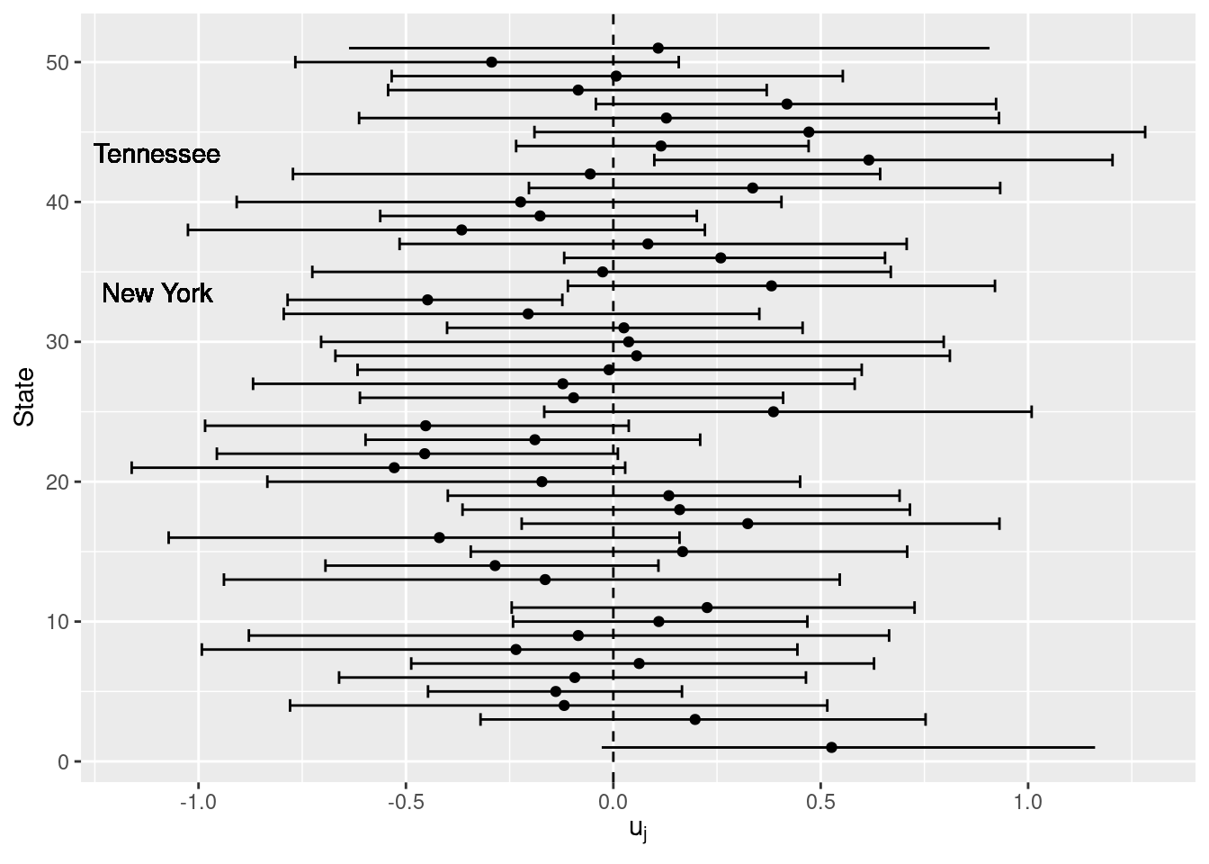
Figure 4.8: Posterior means and 95% credible intervals of the random effects of the US States.

Furthermore, Figure 4.9 shows a map of the point estimates of the state-level random effects, which has been created with packages sf (Pebesma 2018) and USAboundaries (Mullen and Bratt 2018).

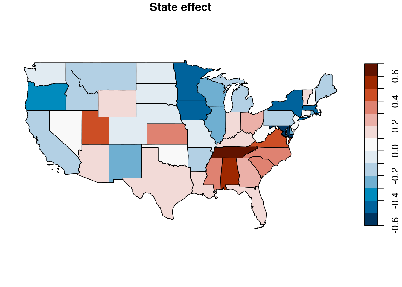
Figure 4.9: Point estimates of state-level random effect.

The map shows an interesting pattern. First of all, the values of the point estimates change smoothly from one state to its neighbors, which may lead us to think that there is some residual spatial variation not explained by the model. For example, several states in the south-east part have positive posterior means of the random effect, which increases the probability of voting for Bush. On the other hand, states on the west coast have a negative point estimate, which makes them have a lower probability of voting for Bush.

4.7 Multilevel models for count data

The next example will discuss the ``stop-and-frisk’’ dataset analyzed in Gelman and Little (1997), Andrew Gelman and Hill (2006) and Gelman, Fagan, and Kiss (2007). This dataset records the number of stops between January 1998 and March 1999 and was used as part of a study to assess whether members of ethnic minorities (in particular, blacks and latinos) were more likely to be stopped by the New York City (NYC) police. Data being analyzed here have been obtained from Prof. Andrew Gelman’s website (see Preface for details), who added some noise to the original data.

Table 4.6 shows the variables in the dataset. The number of stops, population and number of arrests in 1997 (as recorded by the Division of Criminal Justice Services, DCJS) is stratified by precinct, ethnicity and type of crime. The dataset contains data for 75 precincts, which excluded precinct 22 as this covers the Central Park area and it has no population. Note that precincts are identified by an index from 1 to 75 and not by their actual NYC precinct number. Furthermore, only three ethnic groups were considered (white, black and latino) because other ethnic groups covered a small percentage of the stops (about 4%) and ambiguities in the classification (Andrew Gelman and Hill 2006).

Table 4.6: Summary of variables in the NYC police stop and frisk dataset.

Variable	Description
stops	Number of stops between January 1998 and March 1999.
pop	Population.
past.arrests	Number of arrests within New York City in 1997.
precinct	Number of precinct (from 1 to 75)
eth	Ethnicity (black, hispanic or white)
crime	Crime type (violent, weapons, property or drug).

Data can be loaded as follows:

nyc.stops <- read.table(file = "data/frisk_with_noise.dat", skip = 6, 
  header = TRUE)

# Add labels to factors
nyc.stops$eth <- as.factor(nyc.stops$eth)
levels(nyc.stops$eth) <- c("black", "hispanic", "white")
nyc.stops$eth <- relevel(nyc.stops$eth, "white")

nyc.stops$crime <- as.factor(nyc.stops$crime)
levels(nyc.stops$crime) <- c("violent", "weapons", "property", "drug")

Note that in the previous code labels have been assigned to factor variables eth and crime. Furthermore, white has been set as the baseline level for variable eth so that this will become the reference level when fitting models to assess any effect of the ethnicity of stops.

Given that we are not interested in crime type, the next step is to aggregate the data by precinct and ethnicity:

nyc.stops.agg <- aggregate(cbind(stops, past.arrests, pop) ~ precinct + eth,
  data = nyc.stops, sum)

# Population is summed 4 times
nyc.stops.agg$pop <- nyc.stops.agg$pop / 4

Note that now the aggregated population per precinct has been divided by 4 in the aggregated dataset because it is added up 4 times.

In this analysis, the focus is on the ethnicity effect to determine whether individuals from ethnic minorities (i.e., black and hispanic) are more likely to be stopped by the NYC police. For this reason, this effect will be included as a fixed effect in the model. Furthermore, precinct will be included as a random effect as we expect variation between precincts as well. Hence, the resulting model is:

\[ \textrm{stops}_{ep} \sim Po(E_{ep}\theta_{ep}) \]

\[ \log(\theta_{ep}) = \beta_0 + \beta_1 \textrm{eth}_{ep}^{\textrm{black}}+ \beta_2 \textrm{eth}_{ep}^{\textrm{hispanic}}+ u_p \]

\[ u_p \sim N(0, \tau_u), i=1,\ldots,75 \]

Here, \(E_{ep}\) will be taken as a reference (e.g., expected) number of stops considering the number of stops in 1997 multiplied by 15/12 because the number of stops is recorded over a period of 15 months (January 1998 to March 1999). Furthermore, this must be introduced as an offset in the log-scale in the model.

Then, the model can be fit as:

nyc.inla <- inla(stops ~ eth + f(precinct, model = "iid"),
  data = nyc.stops.agg, offset = log((15 / 12) * past.arrests),
  family = "poisson")

summary(nyc.inla)

## 
## Call:
##    c("inla(formula = stops ~ eth + f(precinct, model = \"iid\"), 
##    family = \"poisson\", ", " data = nyc.stops.agg, offset = 
##    log((15/12) * past.arrests))" ) 
## Time used:
##     Pre = 0.226, Running = 0.125, Post = 0.0197, Total = 0.371 
## Fixed effects:
##               mean    sd 0.025quant 0.5quant 0.975quant   mode kld
## (Intercept) -1.088 0.071     -1.227   -1.087     -0.949 -1.087   0
## ethblack     0.418 0.009      0.400    0.418      0.437  0.418   0
## ethhispanic  0.429 0.010      0.410    0.429      0.448  0.429   0
## 
## Random effects:
##   Name     Model
##     precinct IID model
## 
## Model hyperparameters:
##                        mean    sd 0.025quant 0.5quant 0.975quant mode
## Precision for precinct 2.77 0.451       1.96     2.75       3.73 2.70
## 
## Expected number of effective parameters(stdev): 77.21(0.028)
## Number of equivalent replicates : 2.91 
## 
## Marginal log-Likelihood:  -2864.03

Andrew Gelman and Hill (2006) and Gelman, Fagan, and Kiss (2007) also propose a model which includes an ethnicity-precinct noise term, which is included as a random effect and has the interpretation of adding an error term to the linear predictor. Fitting this model requires a new index for each ethnicity-precinct, with different values for each row, and the model is fitted as follows:

# Ethnicity precinct index
nyc.stops.agg$ID <- 1:nrow(nyc.stops.agg)
nyc.inla2 <- inla(stops ~ eth + f(precinct, model = "iid") + 
    f(ID, model = "iid"), 
  data = nyc.stops.agg, offset = log((15/12) * past.arrests),
  family = "poisson")

summary(nyc.inla2)

## 
## Call:
##    c("inla(formula = stops ~ eth + f(precinct, model = \"iid\") + 
##    f(ID, ", " model = \"iid\"), family = \"poisson\", data = 
##    nyc.stops.agg, ", " offset = log((15/12) * past.arrests))") 
## Time used:
##     Pre = 0.269, Running = 0.256, Post = 0.0256, Total = 0.55 
## Fixed effects:
##               mean    sd 0.025quant 0.5quant 0.975quant   mode kld
## (Intercept) -1.214 0.079     -1.369   -1.214     -1.059 -1.214   0
## ethblack     0.497 0.050      0.399    0.497      0.596  0.497   0
## ethhispanic  0.516 0.050      0.417    0.516      0.615  0.516   0
## 
## Random effects:
##   Name     Model
##     precinct IID model
##    ID IID model
## 
## Model hyperparameters:
##                         mean    sd 0.025quant 0.5quant 0.975quant  mode
## Precision for precinct  2.81 0.497       1.94     2.78       3.89  2.72
## Precision for ID       11.87 1.540       9.07    11.79      15.11 11.66
## 
## Expected number of effective parameters(stdev): 213.93(1.10)
## Number of equivalent replicates : 1.05 
## 
## Marginal log-Likelihood:  -1477.90

In both models ethnic minority groups show a clear effect to be stopped more often than white people. Regarding the precinct-level effect, posterior means and 95% credible intervals for each precinct are shown in Figure 4.10. It is clear that some precincts have a number of stops that are higher than the average in 1997 and considering ethnicity.

These results can nicely be plotted in a map using the precinct boundaries provided in the web of the City of New York (see Preface for details). Precinct 121, which was not in 1999, has been merged together with Precinct 122, but this provides slightly different results from the current boundaries of precincts 120 and 122 in Staten Islands, but this is enough for our purpose. Note that Precinct 22 in Central Park has been excluded, so that the map ends with the 75 precincts discussed in the analysis in Andrew Gelman and Hill (2006) and Gelman, Fagan, and Kiss (2007).

Furthermore, precincts in the original dataset have been matched to the NYC precinct number by using the proportion of ethnic groups in each precinct as precinct ids in the original data ranged from 1 to 75. These precinct-level data have been obtained from the original “stop-and-frisk” report (New York Attorney General 1999). This way, we have been able to match each precinct in the original dataset to its actual NYC precinct number. It turned out that precincts in the “stop-and-frisk” dataset were already ordered by NYC precinct number (after excluding Precinct 22 and merging Precincts 121 and 122).

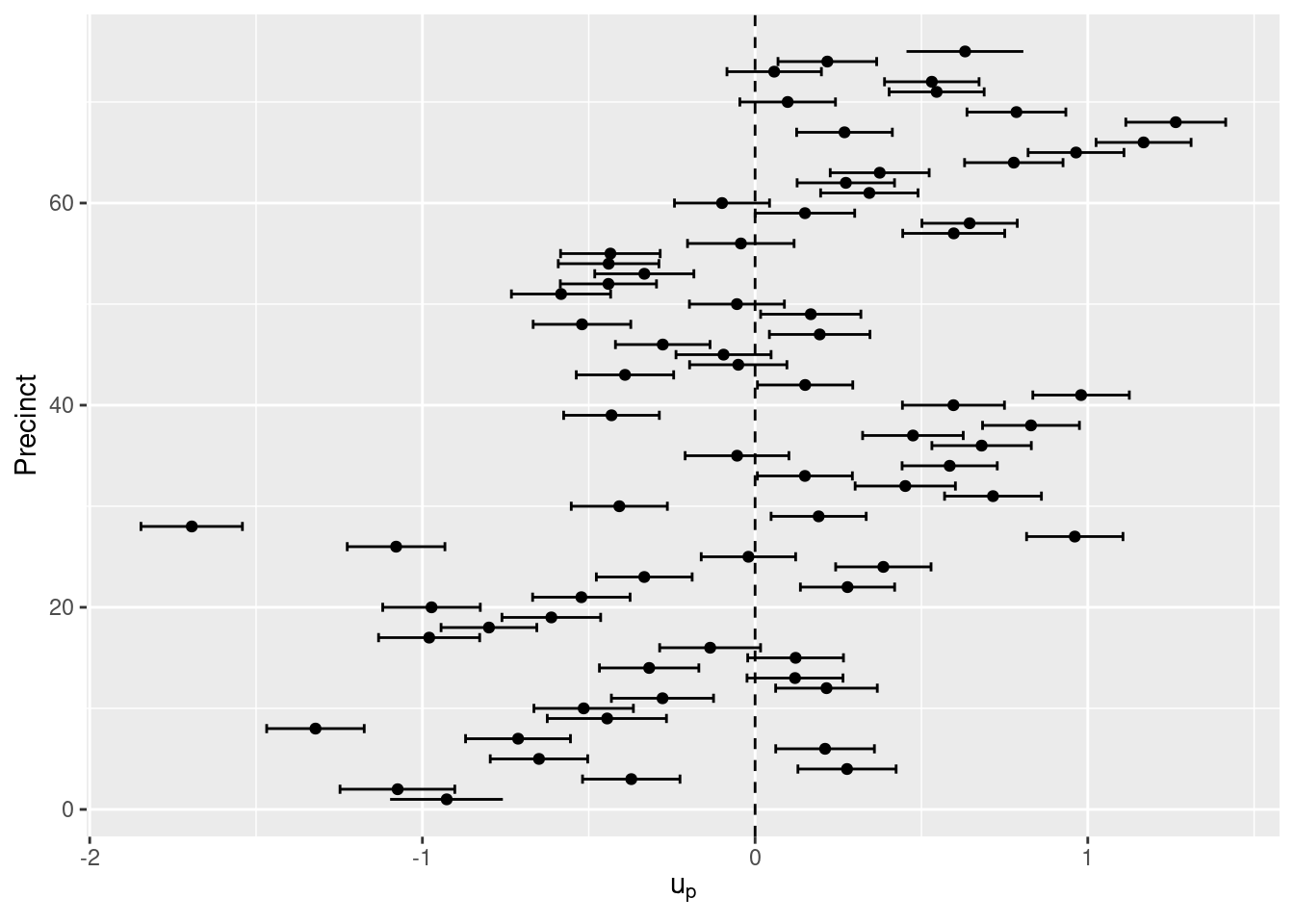
Figure 4.10: Posterior means and 95% credible intervals of the random effects of the 75 NYC precincts.

The next lines of code will load the precinct-level data available as Table I.A.1 in the report New York Attorney General (1999) that records NYC police stop rates by precinct from January 1998 to March 1999:

# Load precinct data
precinct99 <- read.csv2(file = "data/precinct_data_98-99.csv")
rownames(precinct99) <- precinct99$Precinct

# Order by precinct number
precinct99 <- precinct99[order(precinct99$Precinct), ]

# Remove Central Park
precinct99 <- subset(precinct99, Precinct != 22)

Next, a shapefile with the boundaries of the 75 precincts is loaded using function readOGR() from package rgdal (R. Bivand, Keitt, and Rowlingson 2019):

# Test to check boundaries of precincts
library("rgdal")
nyc.precincts <- readOGR("data/Police_Precincts", "nyc_precincts")

The shapefile includes the precinct number in a column. We will assign it as the polygon id in order to merge the SpatialPolygons object to our data:

# Set IDs to polygons
for(i in 1:length(nyc.precincts)) {
  slot(slot(nyc.precincts, "polygons")[[i]], "ID") <- 
    as.character(nyc.precincts$precinct[i])
}

Finally, a SpatialPolygonsDataFrame is created by merging the precinct boundaries to the precinct99 data:

#Merge boundaries and 1999 data
nyc.precincts99 <- SpatialPolygonsDataFrame(nyc.precincts, precinct99)

Then, point estimates of the precinct random effect (e.g., posterior means) can be added to the map in a simple way:

# Add r. eff. estimates
nyc.precincts99$u <- nyc.inla$summary.random$precinct$mean

Note that this is only possible because the order of the precincts is the same in the SpatialPolygonsDataFrame and our fit model. Figure 4.11 shows the point estimates of the random effects for the precincts.

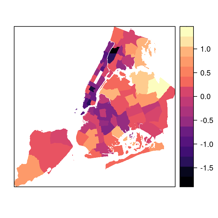
Figure 4.11: Point estimates of the random effects of the 75 precincts of NYC in 1999.

References

Bates, Douglas, Martin Mächler, Ben Bolker, and Steve Walker. 2015. “Fitting Linear Mixed-Effects Models Using lme4.” Journal of Statistical Software 67 (1): 1–48. https://doi.org/10.18637/jss.v067.i01.

Bates, Douglas, and Martin Maechler. 2019. Matrix: Sparse and Dense Matrix Classes and Methods. https://CRAN.R-project.org/package=Matrix.

Belenky, Gregory, Nancy J. Wesensten, David R. Thorne, Maria L. Thomas, Helen C. Sing, Daniel P. Redmond, Michael B. Russo, and Thomas J. Balkin. 2003. “Patterns of Performance Degradation and Restoration During Sleep Restriction and Subsequent Recovery: A Sleep Dose-Response Study.” Journal of Sleep Research 12 (1): 1–12.

Bivand, Roger, Tim Keitt, and Barry Rowlingson. 2019. Rgdal: Bindings for the ’Geospatial’ Data Abstraction Library. https://CRAN.R-project.org/package=rgdal.

Blatchford, P., H. Goldstein, Martin C., and W. Browne. 2002. “A Study of Class Size Effects in English School Reception Year Classes.” British Educational Research Journal 28: 169–85.

Bliese, Paul. 2016. Multilevel: Multilevel Functions. https://CRAN.R-project.org/package=multilevel.

Bliss, C. I. 1967. Statistics in Biology. McGraw Hill, New York.

Box, G., W. Hunter, and J. Hunter. 1978. Statistics for Experimenters. Wiley, New York.

Carpenter, James, Harvey Goldstein, and Michael Kenward. 2011. “REALCOM-Impute Software for Multilevel Multiple Imputation with Mixed Response Types.” Journal of Statistical Software, Articles 45 (5): 1–14. https://doi.org/10.18637/jss.v045.i05.

Faraway, J. 2006. Extending the Linear Model with R. Chapman; Hall, London.

Faraway, Julian. 2016. Faraway: Functions and Datasets for Books by Julian Faraway. https://CRAN.R-project.org/package=faraway.

Faraway, Julian J. 2019a. “Inferential Methods for Linear Mixed Models.” http://www.maths.bath.ac.uk/~jjf23/mixchange/index.html#worked-examples.

Faraway, Julian J. 2019b. “INLA for Linear Mixed Models.” http://www.maths.bath.ac.uk/~jjf23/inla/.

Gelman, A. 2006. “Prior Distributions for Variance Parameters in Hierarchical Models.” Bayesian Analysis 1 (3): 515–34.

Gelman, Andrew, Jeffrey Fagan, and Alex Kiss. 2007. “An Analysis of the New York City Police Department’s ‘Stop-and-Frisk’ Policy in the Context of Claims of Racial Bias.” Journal of the American Statistical Association 102 (479): 813–23.

Gelman, Andrew, and Jennifer Hill. 2006. Data Analysis Using Regression and Multilevel/Hierarchical Models. Cambridge University Press.

Gelman, Andrew, and Thomas C. Little. 1997. “Poststratification into Many Categories Using Hierarchical Logistic Regression.” Survey Methodology 23: 127–35.

Goldstein, Harvey. 2003. Multilevel Statistical Models. 3rd ed. Kendall’s Library of Statistics. Arnold, London.

Jovanovic, Mladen. 2015. “R Playbook: Introduction to Mixed-Models. Multilevel Models Playbook.” http://complementarytraining.net/r-playbook-introduction-to-multilevelhierarchical-models/.

Mullen, Lincoln A., and Jordan Bratt. 2018. “USAboundaries: Historical and Contemporary Boundaries of the United States of America.” Journal of Open Source Software 3 (23): 314. https://doi.org/10.21105/joss.00314.

New York Attorney General. 1999. “The New York Police Department’s ‘Stop and Frisk’ Practices.” https://ag.ny.gov/sites/default/files/pdfs/bureaus/civil_rights/stp_frsk.pdf.

Pebesma, Edzer. 2018. “Simple Features for R: Standardized Support for Spatial Vector Data.” The R Journal 10 (1): 439–46. https://doi.org/10.32614/RJ-2018-009.

Pinheiro, Jose, Douglas Bates, Saikat DebRoy, Deepayan Sarkar, and R Core Team. 2018. nlme: Linear and Nonlinear Mixed Effects Models. https://CRAN.R-project.org/package=nlme.